Watch Now This tutorial has a related video course created by the Real Python team. Watch it together with the written tutorial to deepen your understanding: Using k-Nearest Neighbors (kNN) in Python
In this tutorial, you’ll get a thorough introduction to the k-Nearest Neighbors (kNN) algorithm in Python. The kNN algorithm is one of the most famous machine learning algorithms and an absolute must-have in your machine learning toolbox. Python is the go-to programming language for machine learning, so what better way to discover kNN than with Python’s famous packages NumPy and scikit-learn!
Below, you’ll explore the kNN algorithm both in theory and in practice. While many tutorials skip the theoretical part and focus only on the use of libraries, you don’t want to be dependent on automated packages for your machine learning. It’s important to learn about the mechanics of machine learning algorithms to understand their potential and limitations.
At the same time, it’s essential to understand how to use an algorithm in practice. With that in mind, in the second part of this tutorial, you’ll focus on the use of kNN in the Python library scikit-learn, with advanced tips for pushing performance to the max.
In this tutorial, you’ll learn how to:
- Explain the kNN algorithm both intuitively and mathematically
- Implement kNN in Python from scratch using NumPy
- Use kNN in Python with scikit-learn
- Tune hyperparameters of kNN using
GridSearchCV - Add bagging to kNN for better performance
Free Bonus: Click here to get access to a free NumPy Resources Guide that points you to the best tutorials, videos, and books for improving your NumPy skills.
Basics of Machine Learning
To get you on board, it’s worth taking a step back and doing a quick survey of machine learning in general. In this section, you’ll get an introduction to the fundamental idea behind machine learning, and you’ll see how the kNN algorithm relates to other machine learning tools.
The general idea of machine learning is to get a model to learn trends from historical data on any topic and be able to reproduce those trends on comparable data in the future. Here’s a diagram outlining the basic machine learning process:
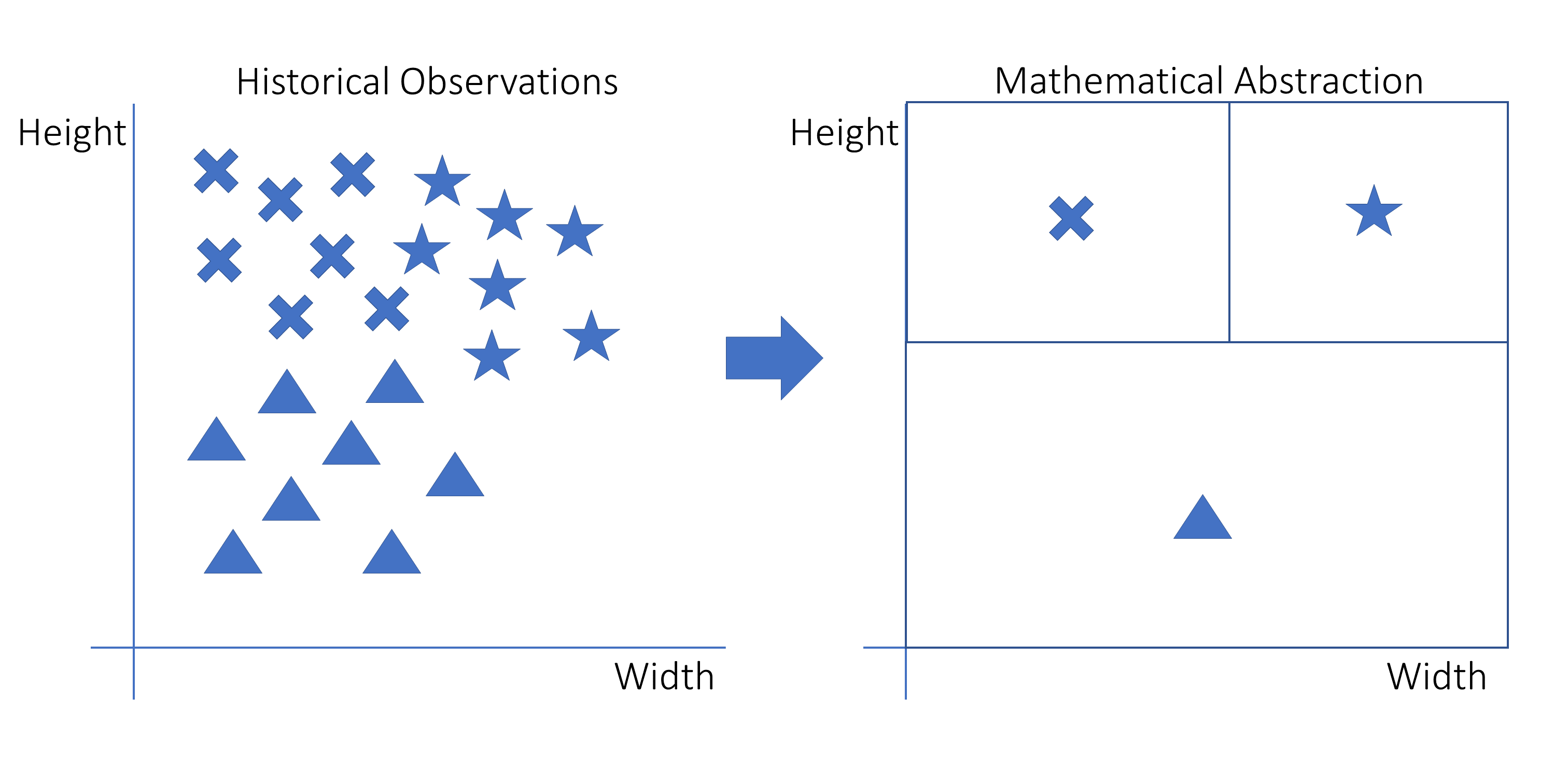
This graph is a visual representation of a machine learning model that is fitted onto historical data. On the left are the original observations with three variables: height, width, and shape. The shapes are stars, crosses, and triangles.
The shapes are located in different areas of the graph. On the right, you see how those original observations have been translated to a decision rule. For a new observation, you need to know the width and the height to determine in which square it falls. The square in which it falls, in turn, defines which shape it is most likely to have.
Many different models could be used for this task. A model is a mathematical formula that can be used to describe data points. One example is the linear model, which uses a linear function defined by the formula y = ax + b.
If you estimate, or fit, a model, you find the optimal values for the fixed parameters using some algorithm. In the linear model, the parameters are a and b. Luckily, you won’t have to invent such estimation algorithms to get started. They’ve already been discovered by great mathematicians.
Once the model is estimated, it becomes a mathematical formula in which you can fill in values for your independent variables to make predictions for your target variable. From a high-level perspective, that’s all that happens!
Distinguishing Features of kNN
Now that you understand the basic idea behind machine learning, the next step is understanding why there are so many models available. The linear model that you just saw is called linear regression.
Linear regression works in some cases but doesn’t always make very precise predictions. That’s why mathematicians have come up with many alternative machine learning models that you can use. The k-Nearest Neighbors algorithm is one of them.
All these models have their peculiarities. If you work on machine learning, you should have a deep understanding of all of them so that you can use the right model in the right situation. To understand why and when to use kNN, you’ll next look at how kNN compares to other machine learning models.
kNN Is a Supervised Machine Learning Algorithm
The first determining property of machine learning algorithms is the split between supervised and unsupervised models. The difference between supervised and unsupervised models is the problem statement.
In supervised models, you have two types of variables at the same time:
- A target variable, which is also called the dependent variable or the
yvariable. - Independent variables, which are also known as
xvariables or explanatory variables.
The target variable is the variable that you want to predict. It depends on the independent variables and it isn’t something that you know ahead of time. The independent variables are variables that you do know ahead of time. You can plug them into an equation to predict the target variable. In this way, it’s relatively similar to the y = ax + b case.
In the graph that you’ve seen before and the following graphs in this section, the target variable is the shape of the data point, and the independent variables are height and width. You can see the idea behind supervised learning in the following graph:

In this graph, the data points each have a height, a width, and a shape. There are crosses, stars, and triangles. On the right is a decision rule that a machine learning model might have learned.
In this case, observations marked with a cross are tall but not wide. Stars are both tall and wide. Triangles are short but can be wide or narrow. Essentially, the model has learned a decision rule to decide whether an observation is more likely to be a cross, a star, or a triangle based only on its height and width.
In unsupervised models, you don’t have a split between target variables and independent variables. Unsupervised learning tries to group data points by evaluating their similarity.
As you can see in the example, you can never be certain that grouped data points fundamentally belong together, but as long as the grouping makes sense, it can be very valuable in practice. You can see the idea behind unsupervised learning in the following graph:

In this graph, the observations don’t have different shapes anymore. They’re all circles. Yet they can still be grouped into three groups based on the distance between points. In this particular example, there are three clusters of points that can be separated based on the empty space between them.
The kNN algorithm is a supervised machine learning model. That means it predicts a target variable using one or multiple independent variables.
To learn more about unsupervised machine learning models, check out K-Means Clustering in Python: A Practical Guide.
kNN Is a Nonlinear Learning Algorithm
A second property that makes a big difference in machine learning algorithms is whether or not the models can estimate nonlinear relationships.
Linear models are models that predict using lines or hyperplanes. In the image, the model is depicted as a line drawn between the points. The model y = ax + b is the classical example of a linear model. You can see how a linear model could fit the example data in the following schematic drawing:

In this picture, the data points are depicted on the left with stars, triangles, and crosses. On the right is a linear model that can separate triangles from non-triangles. The decision is a line. Every point above the line is a non-triangle, and everything below the line is a triangle.
If you wanted to add another independent variable to the previous graph, you would need to draw it as an additional dimension, thereby creating a cube with the shapes inside it. Yet a line wouldn’t be able to cut a cube into two parts. The multidimensional counterpart of the line is the hyperplane. A linear model is therefore represented by a hyperplane, which in the case of two-dimensional space happens to be a line.
Nonlinear models are models that use any approach other than a line to separate their cases. A well-known example is the decision tree, which is basically a long list of if … else statements. In the nonlinear graph, if … else statements would allow you to draw squares or any other form that you wanted to draw. The following graph depicts a nonlinear model applied to the example data:

This graph shows how a decision can be nonlinear. The decision rule is made up of three squares. The box in which a new data point falls will define its predicted shape. Note that it’s not possible to fit this at once using a line: Two lines are needed. This model could be re-created with if … else statements as follows:
- If the data point’s height is low, then it’s a triangle.
- Else, if the data point’s width is low, then it’s a cross.
- Else, if none of the above is true, then it’s a star.
kNN is an example of a nonlinear model. Later in this tutorial, you’ll get back to the exact way that the model is computed.
kNN Is a Supervised Learner for Both Classification and Regression
Supervised machine learning algorithms can be split into two groups based on the type of target variable that they can predict:
-
Classification is a prediction task with a categorical target variable. Classification models learn how to classify any new observation. This assigned class can be either right or wrong, not in between. A classic example of classification is the iris dataset, in which you use physical measurements of plants to predict their species. A famous algorithm that can be used for classification is logistic regression.
-
Regression is a prediction task in which the target variable is numeric. A famous example of regression is the Housing Prices Challenge on Kaggle. In this machine learning contest, participants try to predict the sales prices of houses based on numerous independent variables.
In the following graphic, you can see what a regression and a classification would look like using the previous example:

The left part of this image is a classification. The target variable is the shape of the observation, which is a categorical variable. The right part is a regression. The target variable is numeric. The decision rules could be exactly the same for the two examples, but their interpretations are different.
For a single prediction, classifications are either right or wrong, while regressions have an error on a continuous scale. Having a numeric error measure is more practical, so many classification models predict not only the class but also the probability of being in either of the classes.
Some models can only do regression, some can only do classification, and some can do both. The kNN algorithm seamlessly adapts to both classification and regression. You’ll learn exactly how this works in the next part of this tutorial.
kNN Is Fast and Interpretable
As a final criterion to characterize machine learning models, you need to take into account model complexity. Machine learning, and especially artificial intelligence, is currently blooming and is being used in many complicated tasks, such as understanding text, images, and speech, or for self-driving cars.
More advanced and complex models like neural networks can probably learn anything that a k-Nearest Neighbors model can. After all, those advanced models are very strong learners. However, be aware that this complexity also has its price. In order to make the models fit to your prediction, you’ll generally spend much more time on development.
You’ll also need much more data to fit a more complex model, and data is not always available. Last but not least, more complex models are more difficult for us humans to interpret, and sometimes this interpretation can be very valuable.
This is where the force of the kNN model lies. It allows its users to understand and interpret what’s happening inside the model, and it’s very fast to develop. This makes kNN a great model for many machine learning use cases that don’t require highly complex techniques.
Drawbacks of kNN
It’s only fair to also be honest about the drawbacks of the kNN algorithm. As touched upon before, the real drawback of kNN is its capacity to adapt to highly complex relationships between independent and dependent variables. kNN is less likely to perform well on advanced tasks like computer vision and natural language processing.
You can try to push the performance of kNN as far as possible, potentially by adding other techniques from machine learning. In the last part of the tutorial, you’ll look at a technique called bagging, which is a way to improve predictive performances. At a certain point of complexity, though, kNN will probably be less effective than other models regardless of the way it was tuned.
Use kNN to Predict the Age of Sea Slugs
To follow along with the coding part, you’ll look at an example dataset for the rest of this tutorial—the Abalone Dataset. This dataset contains age measurements on a large number of abalones. Just for information, this is what an abalone looks like:

Abalones are small sea snails that look a bit like mussels. If you want to learn more about them, you can check the abalone Wikipedia page for more information.
The Abalone Problem Statement
The age of an abalone can be found by cutting its shell and counting the number of rings on the shell. In the Abalone Dataset, you can find the age measurements of a large number of abalones along with a lot of other physical measurements.
The goal of the project is to develop a model that can predict the age of an abalone based purely on the other physical measurements. This would allow researchers to estimate the abalone’s age without having to cut its shell and count the rings.
You’ll be applying a kNN to find the closest prediction score possible.
Importing the Abalone Dataset
In this tutorial, you’ll work with the Abalone Dataset. You could download it and use pandas to import the data into Python, but it’s even faster to let pandas import the data directly for you.
To follow along with the code in this tutorial, it is recommended to install Python with Anaconda. The Anaconda distribution comes with many important packages for data science. For more help with setting up your environment, you can check out Setting Up Python for Machine Learning on Windows.
You can import the data using pandas as follows:
>>> import pandas as pd
>>> url = (
...     "https://archive.ics.uci.edu/ml/machine-learning-databases"
...     "/abalone/abalone.data"
... )
>>> abalone = pd.read_csv(url, header=None)
In this code, you first import pandas, then you use it to read the data. You specify the path to be a URL so the file will be fetched directly over the Internet.
To make sure that you’ve imported the data correctly, you can do a quick check as follows:
>>> abalone.head()
   0      1      2      3       4       5       6      7   8
0  M  0.455  0.365  0.095  0.5140  0.2245  0.1010  0.150  15
1  M  0.350  0.265  0.090  0.2255  0.0995  0.0485  0.070   7
2  F  0.530  0.420  0.135  0.6770  0.2565  0.1415  0.210   9
3  M  0.440  0.365  0.125  0.5160  0.2155  0.1140  0.155  10
4  I  0.330  0.255  0.080  0.2050  0.0895  0.0395  0.055   7
This should show you the first five lines of the Abalone Dataset, imported in Python as a pandas DataFrame. You can see that the column names are still missing. You can find those names in the abalone.names file on the UCI machine learning repository. You can add them to your DataFrame as follows:
>>> abalone.columns = [
...     "Sex",
...     "Length",
...     "Diameter",
...     "Height",
...     "Whole weight",
...     "Shucked weight",
...     "Viscera weight",
...     "Shell weight",
...     "Rings",
... ]
The imported data should now be more understandable. But there’s one other thing that you should do: You should remove the Sex column. The goal of the current exercise is to use physical measurements to predict the age of the abalone. Since sex is not a purely physical measure, you should remove it from the dataset. You can delete the Sex column using .drop:
>>> abalone = abalone.drop("Sex", axis=1)
With this code, you delete the Sex column, as it will have no added value in the modeling.
Descriptive Statistics From the Abalone Dataset
When working on machine learning, you need to have an idea of the data you’re working with. Without going into too much depth, here’s a look at some exploratory statistics and graphs.
The target variable of this exercise is Rings, so you can start with that. A histogram will give you a quick and useful overview of the age ranges that you can expect:
>>> import matplotlib.pyplot as plt
>>> abalone["Rings"].hist(bins=15)
>>> plt.show()
This code uses the pandas plotting functionality to generate a histogram with fifteen bins. The decision to use fifteen bins is based on a few trials. When defining the number of bins, you generally try to have neither too many observations per bin nor too few. Too few bins can hide certain patterns, while too many bins can make the histogram lack smoothness. You can see the histogram in the following graph:

The histogram shows that most abalones in the dataset have between five and fifteen rings, but that it’s possible to get up to twenty-five rings. The older abalones are underrepresented in this dataset. This seems intuitive, as age distributions are generally skewed like this due to natural processes.
A second relevant exploration is to find out which of the variables, if any, have a strong correlation with the age. A strong correlation between an independent variable and your goal variable would be a good sign, as this would confirm that physical measurements and age are related.
You can observe the complete correlation matrix in correlation_matrix. The most important correlations are the ones with the target variable Rings. You can get those correlations like this:
>>> correlation_matrix = abalone.corr()
>>> correlation_matrix["Rings"]
Length            0.556720
Diameter          0.574660
Height            0.557467
Whole weight      0.540390
Shucked weight    0.420884
Viscera weight    0.503819
Shell weight      0.627574
Rings             1.000000
Name: Rings, dtype: float64
Now look at the correlation coefficients for Rings with the other variables. The closer they are to 1, the more correlation there is.
You can conclude that there’s at least some correlation between physical measurements of adult abalones and their age, yet it’s also not very high. Very high correlations mean that you can expect a straightforward modeling process. In this case, you’ll have to try and see what results you can obtain using the kNN algorithm.
There are many more possibilities for data exploration using pandas. To learn more about data exploration with pandas, check out Using pandas and Python to Explore Your Dataset.
A Step-by-Step kNN From Scratch in Python
In this part of the tutorial, you’re going to discover how the kNN algorithm works deep down. The algorithm has two main mathematical components that you’ll need to understand. To warm up, you’ll start with a plain English walkthrough of the kNN algorithm.
Plain English Walkthrough of the kNN Algorithm
The kNN algorithm is a little bit atypical as compared to other machine learning algorithms. As you saw earlier, each machine learning model has its specific formula that needs to be estimated. The specificity of the k-Nearest Neighbors algorithm is that this formula is computed not at the moment of fitting but rather at the moment of prediction. This isn’t the case for most other models.
When a new data point arrives, the kNN algorithm, as the name indicates, will start by finding the nearest neighbors of this new data point. Then it takes the values of those neighbors and uses them as a prediction for the new data point.
As an intuitive example of why this works, think of your neighbors. Your neighbors are often relatively similar to you. They’re probably in the same socioeconomic class as you. Maybe they have the same type of work as you, maybe their children go to the same school as yours, and so on. But for some tasks, this kind of approach is not as useful. For instance, it wouldn’t make any sense to look at your neighbor’s favorite color to predict yours.
The kNN algorithm is based on the notion that you can predict the features of a data point based on the features of its neighbors. In some cases, this method of prediction may be successful, while in other cases it may not. Next, you’ll look at the mathematical description of “nearest” for data points and the methods to combine multiple neighbors into one prediction.
Define “Nearest” Using a Mathematical Definition of Distance
To find the data points that are closest to the point that you need to predict, you can use a mathematical definition of distance called Euclidean distance.
To get to this definition, you should first understand what is meant by the difference of two vectors. Here’s an example:
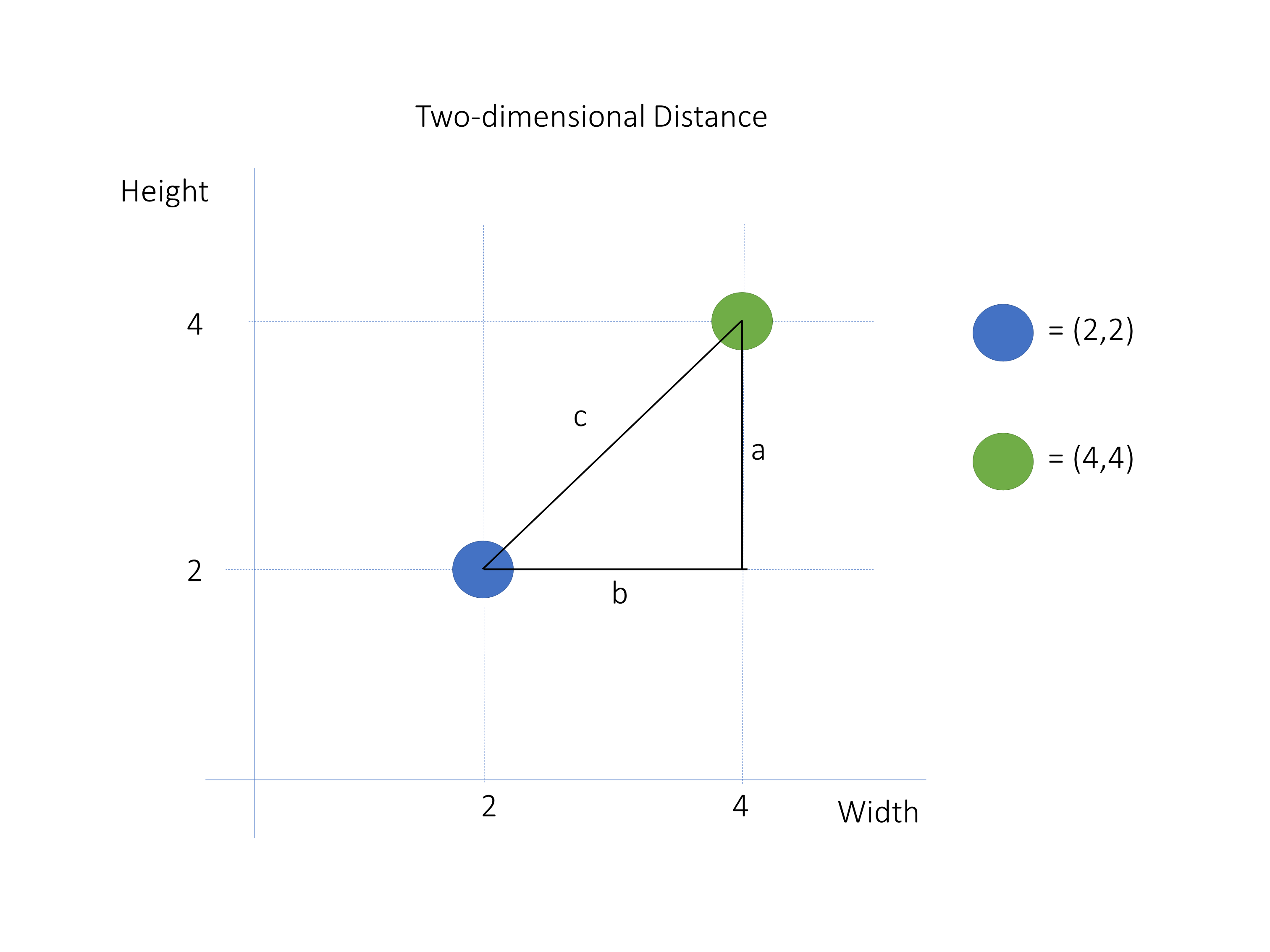
In this picture, you see two data points: blue at (2,2) and green at (4,4). To compute the distance between them, you can start by adding two vectors. Vector a goes from point (4,2) to point (4,4), and vector b goes from point (4,2) to point (2,2). Their heads are indicated by the colored points. Note that they are at a 90 degree angle.
The difference between these vectors is the vector c, which goes from the head of vector a to the head of vector b. The length of vector c represents the distance between your two data points.
The length of a vector is called the norm. The norm is a positive value that indicates the magnitude of the vector. You can compute the norm of a vector using the Euclidean formula:
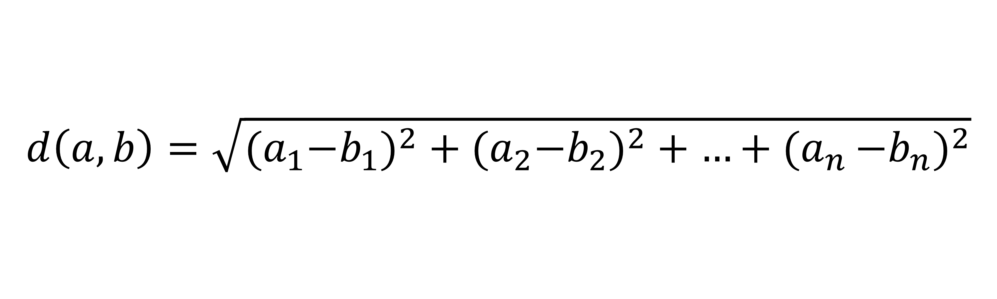
In this formula, the distance is computed by taking the squared differences in each dimension and then taking the square root of the sum of those values. In this case, you should compute the norm of the difference vector c to obtain the distance between the data points.
Now, to apply this to your data, you must understand that your data points are actually vectors. You can then compute the distance between them by computing the norm of the difference vector.
You can compute this in Python using linalg.norm() from NumPy. Here’s an example:
>>> import numpy as np
>>> a = np.array([2, 2])
>>> b = np.array([4, 4])
>>> np.linalg.norm(a - b)
2.8284271247461903
In this code block, you define your data points as vectors. You then compute norm() on the difference between two data points. This way, you directly obtain the distance between two multidimensional points. Even though the points are multidimensional, the distance between them is still a scalar, or a single value.
In case you want to get more details on the math, you can have a look at the Pythagorean theorem to understand how the Euclidean distance formula is derived.
Find the k Nearest Neighbors
Now that you have a way to compute the distance from any point to any point, you can use this to find the nearest neighbors of a point on which you want to make a prediction.
You need to find a number of neighbors, and that number is given by k. The minimum value of k is 1. This means using only one neighbor for the prediction. The maximum is the number of data points that you have. This means using all neighbors. The value of k is something that the user defines. Optimization tools can help you with this, as you’ll see in the last part of this tutorial.
Now, to find the nearest neighbors in NumPy, go back to the Abalone Dataset. As you’ve seen, you need to define distances on the vectors of the independent variables, so you should first get your pandas DataFrame into a NumPy array using the .values attribute:
>>> X = abalone.drop("Rings", axis=1)
>>> X = X.values
>>> y = abalone["Rings"]
>>> y = y.values
This code block generates two objects that now contain your data: X and y. X is the independent variables and y is the dependent variable of your model. Note that you use a capital letter for X but a lowercase letter for y. This is often done in machine learning code because mathematical notation generally uses a capital letter for matrices and a lowercase letter for vectors.
Now you can apply a kNN with k = 3 on a new abalone that has the following physical measurements:
| Variable | Value |
|---|---|
| Length | 0.569552 |
| Diameter | 0.446407 |
| Height | 0.154437 |
| Whole weight | 1.016849 |
| Shucked weight | 0.439051 |
| Viscera weight | 0.222526 |
| Shell weight | 0.291208 |
You can create the NumPy array for this data point as follows:
>>> new_data_point = np.array([
...     0.569552,
...     0.446407,
...     0.154437,
...     1.016849,
...     0.439051,
...     0.222526,
...     0.291208,
... ])
The next step is to compute the distances between this new data point and each of the data points in the Abalone Dataset using the following code:
>>> distances = np.linalg.norm(X - new_data_point, axis=1)
You now have a vector of distances, and you need to find out which are the three closest neighbors. To do this, you need to find the IDs of the minimum distances. You can use a method called .argsort() to sort the array from lowest to highest, and you can take the first k elements to obtain the indices of the k nearest neighbors:
>>> k = 3
>>> nearest_neighbor_ids = distances.argsort()[:k]
>>> nearest_neighbor_ids
array([4045, 1902, 1644], dtype=int32)
This tells you which three neighbors are closest to your new_data_point. In the next paragraph, you’ll see how to convert those neighbors in an estimation.
Voting or Averaging of Multiple Neighbors
Having identified the indices of the three nearest neighbors of your abalone of unknown age, you now need to combine those neighbors into a prediction for your new data point.
As a first step, you need to find the ground truths for those three neighbors:
>>> nearest_neighbor_rings = y[nearest_neighbor_ids]
>>> nearest_neighbor_rings
array([ 9, 11, 10])
Now that you have the values for those three neighbors, you’ll combine them into a prediction for your new data point. Combining the neighbors into a prediction works differently for regression and classification.
Average for Regression
In regression problems, the target variable is numeric. You combine multiple neighbors into one prediction by taking the average of their values of the target variable. You can do this as follows:
>>> prediction = nearest_neighbor_rings.mean()
You’ll get a value of 10 for prediction. This means that the 3-Nearest Neighbor prediction for your new data point is 10. You could do the same for any number of new abalones that you want.
Mode for Classification
In classification problems, the target variable is categorical. As discussed before, you can’t take averages on categorical variables. For example, what would be the average of three predicted car brands? That would be impossible to say. You can’t apply an average on class predictions.
Instead, in the case of classification, you take the mode. The mode is the value that occurs most often. This means that you count the classes of all the neighbors, and you retain the most common class. The prediction is the value that occurs most often among the neighbors.
If there are multiple modes, there are multiple possible solutions. You could select a final winner randomly from the winners. You could also make the final decision based on the distances of the neighbors, in which case the mode of the closest neighbors would be retained.
You can compute the mode using the SciPy mode() function. As the abalone example is not a case of classification, the following code shows how you can compute the mode for a toy example:
>>> import scipy.stats
>>> class_neighbors = np.array(["A", "B", "B", "C"])
>>> scipy.stats.mode(class_neighbors)
ModeResult(mode=array(['B'], dtype='<U1'), count=array([2]))
As you can see, the mode in this example is "B" because it’s the value that occurs most often in the input data.
Fit kNN in Python Using scikit-learn
While coding an algorithm from scratch is great for learning purposes, it’s usually not very practical when working on a machine learning task. In this section, you’ll explore the implementation of the kNN algorithm used in scikit-learn, one of the most comprehensive machine learning packages in Python.
Splitting Data Into Training and Test Sets for Model Evaluation
In this section, you’ll evaluate the quality of your abalone kNN model. In the previous sections, you had a technical focus, but you’re now going to have a more pragmatic and results-oriented point of view.
There are multiple ways of evaluating models, but the most common one is the train-test split. When using a train-test split for model evaluation, you split the dataset into two parts:
- Training data is used to fit the model. For kNN, this means that the training data will be used as neighbors.
- Test data is used to evaluate the model. It means that you’ll make predictions for the number of rings of each of the abalones in the test data and compare those results to the known true number of rings.
You can split the data into training and test sets in Python using scikit-learn’s built-in train_test_split():
>>> from sklearn.model_selection import train_test_split
>>> X_train, X_test, y_train, y_test = train_test_split(
...     X, y, test_size=0.2, random_state=12345
... )
The test_size refers to the number of observations that you want to put in the training data and the test data. If you specify a test_size of 0.2, your test_size will be 20 percent of the original data, therefore leaving the other 80 percent as training data.
The random_state is a parameter that allows you to obtain the same results every time the code is run. train_test_split() makes a random split in the data, which is problematic for reproducing the results. Therefore, it’s common to use random_state. The choice of value in random_state is arbitrary.
In the above code, you separate the data into training and test data. This is needed for objective model evaluation. You can now proceed to fit a kNN model on the training data using scikit-learn.
Fitting a kNN Regression in scikit-learn to the Abalone Dataset
To fit a model from scikit-learn, you start by creating a model of the correct class. At this point, you also need to choose the values for your hyperparameters. For the kNN algorithm, you need to choose the value for k, which is called n_neighbors in the scikit-learn implementation. Here’s how you can do this in Python:
>>> from sklearn.neighbors import KNeighborsRegressor
>>> knn_model = KNeighborsRegressor(n_neighbors=3)
You create an unfitted model with knn_model. This model will use the three nearest neighbors to predict the value of a future data point. To get the data into the model, you can then fit the model on the training dataset:
>>> knn_model.fit(X_train, y_train)
Using .fit(), you let the model learn from the data. At this point, knn_model contains everything that’s needed to make predictions on new abalone data points. That’s all the code you need for fitting a kNN regression using Python!
Using scikit-learn to Inspect Model Fit
Fitting a model, however, isn’t enough. In this section, you’ll look at some functions that you can use to evaluate the fit.
There are many evaluation metrics available for regression, but you’ll use one of the most common ones, the root-mean-square error (RMSE). The RMSE of a prediction is computed as follows:
- Compute the difference between each data point’s actual value and predicted value.
- For each difference, take the square of this difference.
- Sum all the squared differences.
- Take the square root of the summed value.
To start, you can evaluate the prediction error on the training data. This means that you use the training data for prediction, so you know that the result should be relatively good. You can use the following code to obtain the RMSE:
>>> from sklearn.metrics import mean_squared_error
>>> from math import sqrt
>>> train_preds = knn_model.predict(X_train)
>>> mse = mean_squared_error(y_train, train_preds)
>>> rmse = sqrt(mse)
>>> rmse
1.65
In this code, you compute the RMSE using the knn_model that you fitted in the previous code block. You compute the RMSE on the training data for now. For a more realistic result, you should evaluate the performances on data that aren’t included in the model. This is why you kept the test set separate for now. You can evaluate the predictive performances on the test set with the same function as before:
>>> test_preds = knn_model.predict(X_test)
>>> mse = mean_squared_error(y_test, test_preds)
>>> rmse = sqrt(mse)
>>> rmse
2.37
In this code block, you evaluate the error on data that wasn’t yet known by the model. This more-realistic RMSE is slightly higher than before. The RMSE measures the average error of the predicted age, so you can interpret this as having, on average, an error of 1.65 years. Whether an improvement from 2.37 years to 1.65 years is good is case specific. At least you’re getting closer to correctly estimating the age.
Until now, you’ve only used the scikit-learn kNN algorithm out of the box. You haven’t yet done any tuning of hyperparameters and a random choice for k. You can observe a relatively large difference between the RMSE on the training data and the RMSE on the test data. This means that the model suffers from overfitting on the training data: It does not generalize well.
This is nothing to worry about at this point. In the next part, you’ll see how to optimize the prediction error or test error using various tuning methods.
Plotting the Fit of Your Model
A last thing to look at before starting to improve the model is the actual fit of your model. To understand what the model has learned, you can visualize how your predictions have been made using Matplotlib:
>>> import seaborn as sns
>>> cmap = sns.cubehelix_palette(as_cmap=True)
>>> f, ax = plt.subplots()
>>> points = ax.scatter(
...     X_test[:, 0], X_test[:, 1], c=test_preds, s=50, cmap=cmap
... )
>>> f.colorbar(points)
>>> plt.show()
In this code block, you use Seaborn to create a scatter plot of the first and second columns of X_test by subsetting the arrays X_test[:,0] and X_test[:,1]. Remember from before that the first two columns are Length and Diameter. They are strongly correlated, as you’ve seen in the correlations table.
You use c to specify that the predicted values (test_preds) should be used as a colorbar. The argument s is used to specify the size of the points in the scatter plot. You use cmap to specify the cubehelix_palette color map. To learn more about plotting with Matplotlib, check out Python Plotting With Matplotlib.
With the above code, you’ll get the following graph:

On this graph, each point is an abalone from the test set, with its actual length and actual diameter on the X- and Y-axis, respectively. The color of the point reflects the predicted age. You can see that the longer and larger an abalone is, the higher its predicted age. This is logical, and it’s a positive sign. It means that your model is learning something that seems correct.
To confirm whether this trend exists in actual abalone data, you can do the same for the actual values by simply replacing the variable that is used for c:
>>> cmap = sns.cubehelix_palette(as_cmap=True)
>>> f, ax = plt.subplots()
>>> points = ax.scatter(
...     X_test[:, 0], X_test[:, 1], c=y_test, s=50, cmap=cmap
>>> )
>>> f.colorbar(points)
>>> plt.show()
This code uses Seaborn to create a scatterplot with a colorbar. It produces the following graph:

This confirms that the trend your model is learning does indeed make sense.
You could extract a visualization for each combination of the seven independent variables. For this tutorial, that would be too long, but don’t hesitate to try it out. The only thing to change is the columns that are specified in the scatter.
These visualizations are two-dimensional views of a seven-dimensional dataset. If you play around with them, it will give you a great understanding of what the model is learning and, maybe, what it’s not learning or is learning wrong.
Tune and Optimize kNN in Python Using scikit-learn
There are numerous ways you can improve your predictive score. Some improvements could be made by working on the input data using data wrangling, but in this tutorial, the focus is on the kNN algorithm. Next, you’ll look at ways to improve the algorithm part of the modeling pipeline.
Improving kNN Performances in scikit-learn Using GridSearchCV
Until now, you’ve always worked with k=3 in the kNN algorithm, but the best value for k is something that you need to find empirically for each dataset.
When you use few neighbors, you have a prediction that will be much more variable than when you use more neighbors:
-
If you use one neighbor only, the prediction can strongly change from one point to the other. When you think about your own neighbors, one may be quite different from the others. If you lived next to an outlier, your 1-NN prediction would be wrong.
-
If you have multiple data points, the impact of one extremely different neighbor will be much less.
-
If you use too many neighbors, the prediction of each point risks being very close. Let’s say that you use all neighbors for a prediction. In that case, every prediction would be the same.
To find the best value for k, you’re going to use a tool called GridSearchCV. This is a tool that is often used for tuning hyperparameters of machine learning models. In your case, it will help by automatically finding the best value of k for your dataset.
GridSearchCV is available in scikit-learn, and it has the benefit of being used in almost the exact same way as the scikit-learn models:
>>> from sklearn.model_selection import GridSearchCV
>>> parameters = {"n_neighbors": range(1, 50)}
>>> gridsearch = GridSearchCV(KNeighborsRegressor(), parameters)
>>> gridsearch.fit(X_train, y_train)
GridSearchCV(estimator=KNeighborsRegressor(),
             param_grid={'n_neighbors': range(1, 50),
                         'weights': ['uniform', 'distance']})
Here, you use GridSearchCV to fit the model. In short, GridSearchCV repeatedly fits kNN regressors on a part of the data and tests the performances on the remaining part of the data. Doing this repeatedly will yield a reliable estimate of the predictive performance of each of the values for k. In this example, you test the values from 1 to 50.
In the end, it will retain the best performing value of k, which you can access with .best_params_:
>>> gridsearch.best_params_
{'n_neighbors': 25, 'weights': 'distance'}
In this code, you print the parameters that have the lowest error score. With .best_params_, you can see that choosing 25 as value for k will yield the best predictive performance. Now that you know what the best value of k is, you can see how it affects your train and test performances:
>>> train_preds_grid = gridsearch.predict(X_train)
>>> train_mse = mean_squared_error(y_train, train_preds_grid)
>>> train_rmse = sqrt(train_mse)
>>> test_preds_grid = gridsearch.predict(X_test)
>>> test_mse = mean_squared_error(y_test, test_preds_grid)
>>> test_rmse = sqrt(test_mse)
>>> train_rmse
2.0731294674202143
>>> test_rmse
2.1700197339962175
With this code, you fit the model on the training data and evaluate the test data. You can see that the training error is worse than before, but the test error is better than before. This means that your model fits less closely to the training data. Using GridSearchCV to find a value for k has reduced the problem of overfitting on the training data.
Adding Weighted Average of Neighbors Based on Distance
Using GridSearchCV, you reduced the test RMSE from 2.37 to 2.17. In this section, you’ll see how to improve the performances even more.
Below, you’ll test whether the performance of your model will be any better when predicting using a weighted average instead of a regular average. This means that neighbors that are further away will less strongly influence the prediction.
You can do this by setting the weights hyperparameter to the value of "distance". However, setting this weighted average could have an impact on the optimal value of k. Therefore, you’ll again use GridSearchCV to tell you which type of averaging you should use:
>>> parameters = {
...     "n_neighbors": range(1, 50),
...     "weights": ["uniform", "distance"],
... }
>>> gridsearch = GridSearchCV(KNeighborsRegressor(), parameters)
>>> gridsearch.fit(X_train, y_train)
GridSearchCV(estimator=KNeighborsRegressor(),
             param_grid={'n_neighbors': range(1, 50),
                         'weights': ['uniform', 'distance']})
>>> gridsearch.best_params_
{'n_neighbors': 25, 'weights': 'distance'}
>>> test_preds_grid = gridsearch.predict(X_test)
>>> test_mse = mean_squared_error(y_test, test_preds_grid)
>>> test_rmse = sqrt(test_mse)
>>> test_rmse
2.163426558494748
Here, you test whether it makes sense to use a different weighing using your GridSearchCV. Applying a weighted average rather than a regular average has reduced the prediction error from 2.17 to 2.1634. Although this isn’t a huge improvement, it’s still better, which makes it worth it.
Further Improving on kNN in scikit-learn With Bagging
As a third step for kNN tuning, you can use bagging. Bagging is an ensemble method, or a method that takes a relatively straightforward machine learning model and fits a large number of those models with slight variations in each fit. Bagging often uses decision trees, but kNN works perfectly as well.
Ensemble methods are often more performant than single models. One model can be wrong from time to time, but the average of a hundred models should be wrong less often. The errors of different individual models are likely to average each other out, and the resulting prediction will be less variable.
You can use scikit-learn to apply bagging to your kNN regression using the following steps. First, create the KNeighborsRegressor with the best choices for k and weights that you got from GridSearchCV:
>>> best_k = gridsearch.best_params_["n_neighbors"]
>>> best_weights = gridsearch.best_params_["weights"]
>>> bagged_knn = KNeighborsRegressor(
...     n_neighbors=best_k, weights=best_weights
... )
Then import the BaggingRegressor class from scikit-learn and create a new instance with 100 estimators using the bagged_knn model:
>>> from sklearn.ensemble import BaggingRegressor
>>> bagging_model = BaggingRegressor(bagged_knn, n_estimators=100)
Now you can make a prediction and calculate the RMSE to see if it improved:
>>> test_preds_grid = bagging_model.predict(X_test)
>>> test_mse = mean_squared_error(y_test, test_preds_grid)
>>> test_rmse = sqrt(test_mse)
>>> test_rmse
2.1616
The prediction error on the bagged kNN is 2.1616, which is slightly smaller than the previous error that you obtained. It does take a little more time to execute, but for this example, that’s not problematic.
Comparison of the Four Models
In three incremental steps, you’ve pushed the predictive performance of the algorithm. The following table shows a recap of the different models and their performances:
| Model | Error |
|---|---|
Arbitrary k |
2.37 |
GridSearchCV for k |
2.17 |
GridSearchCV for k and weights |
2.1634 |
Bagging and GridSearchCV |
2.1616 |
In this table, you see the four models from simplest to most complex. The order of complexity corresponds with the order of the error metrics. The model with a random k performed the worst, and the model with the bagging and GridSearchCV performed the best.
More improvement may be possible for abalone predictions. For instance, it would be possible to look for ways to wrangle the data differently or to find other external data sources.
Conclusion
Now that you know all about the kNN algorithm, you’re ready to start building performant predictive models in Python. It takes a few steps to move from a basic kNN model to a fully tuned model, but the performance increase is totally worth it!
In this tutorial you learned how to:
- Understand the mathematical foundations behind the kNN algorithm
- Code the kNN algorithm from scratch in NumPy
- Use the scikit-learn implementation to fit a kNN with a minimal amount of code
- Use
GridSearchCVto find the best kNN hyperparameters - Push kNN to its maximum performance using bagging
A great thing about model-tuning tools is that many of them are not only applicable to the kNN algorithm, but they also apply to many other machine learning algorithms. To continue your machine learning journey, check out the Machine Learning Learning Path, and feel free to leave a comment to share any questions or remarks that you may have.
Watch Now This tutorial has a related video course created by the Real Python team. Watch it together with the written tutorial to deepen your understanding: Using k-Nearest Neighbors (kNN) in Python