
Linear programming is a set of techniques used in mathematical programming, sometimes called mathematical optimization, to solve systems of linear equations and inequalities while maximizing or minimizing some linear function. It’s important in fields like scientific computing, economics, technical sciences, manufacturing, transportation, military, management, energy, and so on.
The Python ecosystem offers several comprehensive and powerful tools for linear programming. You can choose between simple and complex tools as well as between free and commercial ones. It all depends on your needs.
In this tutorial, you’ll learn:
- What linear programming is and why it’s important
- Which Python tools are suitable for linear programming
- How to build a linear programming model in Python
- How to solve a linear programming problem with Python
You’ll first learn about the fundamentals of linear programming. Then you’ll explore how to implement linear programming techniques in Python. Finally, you’ll look at resources and libraries to help further your linear programming journey.
Free Bonus: 5 Thoughts On Python Mastery, a free course for Python developers that shows you the roadmap and the mindset you’ll need to take your Python skills to the next level.
Linear Programming Explanation
In this section, you’ll learn the basics of linear programming and a related discipline, mixed-integer linear programming. In the next section, you’ll see some practical linear programming examples. Later, you’ll solve linear programming and mixed-integer linear programming problems with Python.
What Is Linear Programming?
Imagine that you have a system of linear equations and inequalities. Such systems often have many possible solutions. Linear programming is a set of mathematical and computational tools that allows you to find a particular solution to this system that corresponds to the maximum or minimum of some other linear function.
What Is Mixed-Integer Linear Programming?
Mixed-integer linear programming is an extension of linear programming. It handles problems in which at least one variable takes a discrete integer rather than a continuous value. Although mixed-integer problems look similar to continuous variable problems at first sight, they offer significant advantages in terms of flexibility and precision.
Integer variables are important for properly representing quantities naturally expressed with integers, like the number of airplanes produced or the number of customers served.
A particularly important kind of integer variable is the binary variable. It can take only the values zero or one and is useful in making yes-or-no decisions, such as whether a plant should be built or if a machine should be turned on or off. You can also use them to mimic logical constraints.
Why Is Linear Programming Important?
Linear programming is a fundamental optimization technique that’s been used for decades in science- and math-intensive fields. It’s precise, relatively fast, and suitable for a range of practical applications.
Mixed-integer linear programming allows you to overcome many of the limitations of linear programming. You can approximate non-linear functions with piecewise linear functions, use semi-continuous variables, model logical constraints, and more. It’s a computationally intensive tool, but the advances in computer hardware and software make it more applicable every day.
Often, when people try to formulate and solve an optimization problem, the first question is whether they can apply linear programming or mixed-integer linear programming.
Some use cases of linear programming and mixed-integer linear programming are illustrated in the following articles:
The importance of linear programming, and especially mixed-integer linear programming, has increased over time as computers have gotten more capable, algorithms have improved, and more user-friendly software solutions have become available.
Linear Programming With Python
The basic method for solving linear programming problems is called the simplex method, which has several variants. Another popular approach is the interior-point method.
Mixed-integer linear programming problems are solved with more complex and computationally intensive methods like the branch-and-bound method, which uses linear programming under the hood. Some variants of this method are the branch-and-cut method, which involves the use of cutting planes, and the branch-and-price method.
There are several suitable and well-known Python tools for linear programming and mixed-integer linear programming. Some of them are open source, while others are proprietary. Whether you need a free or paid tool depends on the size and complexity of your problem as well as on the need for speed and flexibility.
It’s worth mentioning that almost all widely used linear programming and mixed-integer linear programming libraries are native to and written in Fortran or C or C++. This is because linear programming requires computationally intensive work with (often large) matrices. Such libraries are called solvers. The Python tools are just wrappers around the solvers.
Python is suitable for building wrappers around native libraries because it works well with C/C++. You’re not going to need any C/C++ (or Fortran) for this tutorial, but if you want to learn more about this cool feature, then check out the following resources:
Basically, when you define and solve a model, you use Python functions or methods to call a low-level library that does the actual optimization job and returns the solution to your Python object.
Several free Python libraries are specialized to interact with linear or mixed-integer linear programming solvers:
In this tutorial, you’ll use SciPy and PuLP to define and solve linear programming problems.
Linear Programming Examples
In this section, you’ll see two examples of linear programming problems:
- A small problem that illustrates what linear programming is
- A practical problem related to resource allocation that illustrates linear programming concepts in a real-world scenario
You’ll use Python to solve these two problems in the next section.
Small Linear Programming Problem
Consider the following linear programming problem:
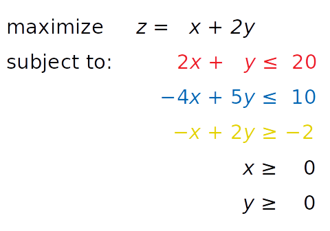
You need to find x and y such that the red, blue, and yellow inequalities, as well as the inequalities x ≥ 0 and y ≥ 0, are satisfied. At the same time, your solution must correspond to the largest possible value of z.
The independent variables you need to find—in this case x and y—are called the decision variables. The function of the decision variables to be maximized or minimized—in this case z—is called the objective function, the cost function, or just the goal. The inequalities you need to satisfy are called the inequality constraints. You can also have equations among the constraints called equality constraints.
This is how you can visualize the problem:
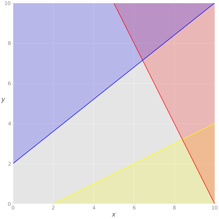
The red line represents the function 2x + y = 20, and the red area above it shows where the red inequality is not satisfied. Similarly, the blue line is the function −4x + 5y = 10, and the blue area is forbidden because it violates the blue inequality. The yellow line is −x + 2y = −2, and the yellow area below it is where the yellow inequality isn’t valid.
If you disregard the red, blue, and yellow areas, only the gray area remains. Each point of the gray area satisfies all constraints and is a potential solution to the problem. This area is called the feasible region, and its points are feasible solutions. In this case, there’s an infinite number of feasible solutions.
You want to maximize z. The feasible solution that corresponds to maximal z is the optimal solution. If you were trying to minimize the objective function instead, then the optimal solution would correspond to its feasible minimum.
Note that z is linear. You can imagine it as a plane in three-dimensional space. This is why the optimal solution must be on a vertex, or corner, of the feasible region. In this case, the optimal solution is the point where the red and blue lines intersect, as you’ll see later.
Sometimes a whole edge of the feasible region, or even the entire region, can correspond to the same value of z. In that case, you have many optimal solutions.
You’re now ready to expand the problem with the additional equality constraint shown in green:
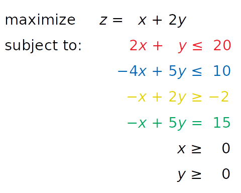
The equation −x + 5y = 15, written in green, is new. It’s an equality constraint. You can visualize it by adding a corresponding green line to the previous image:
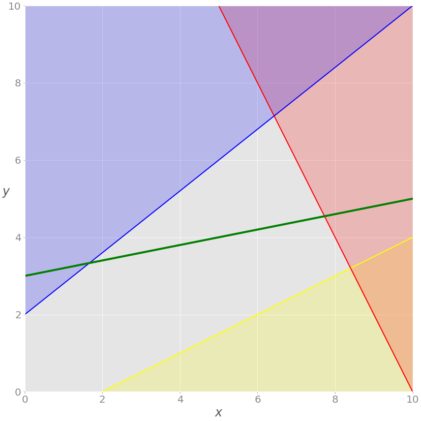
The solution now must satisfy the green equality, so the feasible region isn’t the entire gray area anymore. It’s the part of the green line passing through the gray area from the intersection point with the blue line to the intersection point with the red line. The latter point is the solution.
If you insert the demand that all values of x must be integers, then you’ll get a mixed-integer linear programming problem, and the set of feasible solutions will change once again:
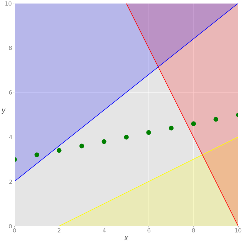
You no longer have the green line, only the points along the line where the value of x is an integer. The feasible solutions are the green points on the gray background, and the optimal one in this case is nearest to the red line.
These three examples illustrate feasible linear programming problems because they have bounded feasible regions and finite solutions.
Infeasible Linear Programming Problem
A linear programming problem is infeasible if it doesn’t have a solution. This usually happens when no solution can satisfy all constraints at once.
For example, consider what would happen if you added the constraint x + y ≤ −1. Then at least one of the decision variables (x or y) would have to be negative. This is in conflict with the given constraints x ≥ 0 and y ≥ 0. Such a system doesn’t have a feasible solution, so it’s called infeasible.
Another example would be adding a second equality constraint parallel to the green line. These two lines wouldn’t have a point in common, so there wouldn’t be a solution that satisfies both constraints.
Unbounded Linear Programming Problem
A linear programming problem is unbounded if its feasible region isn’t bounded and the solution is not finite. This means that at least one of your variables isn’t constrained and can reach to positive or negative infinity, making the objective infinite as well.
For example, say you take the initial problem above and drop the red and yellow constraints. Dropping constraints out of a problem is called relaxing the problem. In such a case, x and y wouldn’t be bounded on the positive side. You’d be able to increase them toward positive infinity, yielding an infinitely large z value.
Resource Allocation Problem
In the previous sections, you looked at an abstract linear programming problem that wasn’t tied to any real-world application. In this subsection, you’ll find a more concrete and practical optimization problem related to resource allocation in manufacturing.
Say that a factory produces four different products, and that the daily produced amount of the first product is x₁, the amount produced of the second product is x₂, and so on. The goal is to determine the profit-maximizing daily production amount for each product, bearing in mind the following conditions:
-
The profit per unit of product is $20, $12, $40, and $25 for the first, second, third, and fourth product, respectively.
-
Due to manpower constraints, the total number of units produced per day can’t exceed fifty.
-
For each unit of the first product, three units of the raw material A are consumed. Each unit of the second product requires two units of the raw material A and one unit of the raw material B. Each unit of the third product needs one unit of A and two units of B. Finally, each unit of the fourth product requires three units of B.
-
Due to the transportation and storage constraints, the factory can consume up to one hundred units of the raw material A and ninety units of B per day.
The mathematical model can be defined like this:
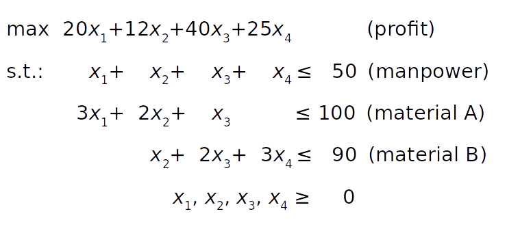
The objective function (profit) is defined in condition 1. The manpower constraint follows from condition 2. The constraints on the raw materials A and B can be derived from conditions 3 and 4 by summing the raw material requirements for each product.
Finally, the product amounts can’t be negative, so all decision variables must be greater than or equal to zero.
Unlike the previous example, you can’t conveniently visualize this one because it has four decision variables. However, the principles remain the same regardless of the dimensionality of the problem.
Linear Programming Python Implementation
In this tutorial, you’ll use two Python packages to solve the linear programming problem described above:
- SciPy is a general-purpose package for scientific computing with Python.
- PuLP is a Python linear programming API for defining problems and invoking external solvers.
SciPy is straightforward to set up. Once you install it, you’ll have everything you need to start. Its subpackage scipy.optimize can be used for both linear and nonlinear optimization.
PuLP allows you to choose solvers and formulate problems in a more natural way. The default solver used by PuLP is the COIN-OR Branch and Cut Solver (CBC). It’s connected to the COIN-OR Linear Programming Solver (CLP) for linear relaxations and the COIN-OR Cut Generator Library (CGL) for cuts generation.
Another great open source solver is the GNU Linear Programming Kit (GLPK). Some well-known and very powerful commercial and proprietary solutions are Gurobi, CPLEX, and XPRESS.
Besides offering flexibility when defining problems and the ability to run various solvers, PuLP is less complicated to use than alternatives like Pyomo or CVXOPT, which require more time and effort to master.
Installing SciPy and PuLP
To follow this tutorial, you’ll need to install SciPy and PuLP. The examples below use version 1.4.1 of SciPy and version 2.1 of PuLP.
You can install both using pip:
$ python -m pip install -U "scipy==1.4.*" "pulp==2.1"
You might need to run pulptest or sudo pulptest to enable the default solvers for PuLP, especially if you’re using Linux or Mac:
$ pulptest
Optionally, you can download, install, and use GLPK. It’s free and open source and works on Windows, MacOS, and Linux. You’ll see how to use GLPK (in addition to CBC) with PuLP later in this tutorial.
On Windows, you can download the archives and run the installation files.
On MacOS, you can use Homebrew:
$ brew install glpk
On Debian and Ubuntu, use apt to install glpk and glpk-utils:
$ sudo apt install glpk glpk-utils
On Fedora, use dnf with glpk-utils:
$ sudo dnf install glpk-utils
You might also find conda useful for installing GLPK:
$ conda install -c conda-forge glpk
After completing the installation, you can check the version of GLPK:
$ glpsol --version
See GLPK’s tutorials on installing with Windows executables and Linux packages for more information.
Using SciPy
In this section, you’ll learn how to use the SciPy optimization and root-finding library for linear programming.
To define and solve optimization problems with SciPy, you need to import scipy.optimize.linprog():
>>> from scipy.optimize import linprog
Now that you have linprog() imported, you can start optimizing.
Example 1
Let’s first solve the linear programming problem from above:
linprog() solves only minimization (not maximization) problems and doesn’t allow inequality constraints with the greater than or equal to sign (≥). To work around these issues, you need to modify your problem before starting optimization:
- Instead of maximizing z = x + 2y, you can minimize its negative(−z = −x − 2y).
- Instead of having the greater than or equal to sign, you can multiply the yellow inequality by −1 and get the opposite less than or equal to sign (≤).
After introducing these changes, you get a new system:
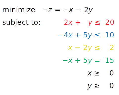
This system is equivalent to the original and will have the same solution. The only reason to apply these changes is to overcome the limitations of SciPy related to the problem formulation.
The next step is to define the input values:
>>> obj = [-1, -2]
>>> #      ─┬  ─┬
>>> #       │   └┤ Coefficient for y
>>> #       └────┤ Coefficient for x

>>> lhs_ineq = [[ 2,  1],  # Red constraint left side
...             [-4,  5],  # Blue constraint left side
...             [ 1, -2]]  # Yellow constraint left side

>>> rhs_ineq = [20,  # Red constraint right side
...             10,  # Blue constraint right side
...              2]  # Yellow constraint right side

>>> lhs_eq = [[-1, 5]]  # Green constraint left side
>>> rhs_eq = [15]       # Green constraint right side
You put the values from the system above into the appropriate lists, tuples, or NumPy arrays:
objholds the coefficients from the objective function.lhs_ineqholds the left-side coefficients from the inequality (red, blue, and yellow) constraints.rhs_ineqholds the right-side coefficients from the inequality (red, blue, and yellow) constraints.lhs_eqholds the left-side coefficients from the equality (green) constraint.rhs_eqholds the right-side coefficients from the equality (green) constraint.
Note: Please, be careful with the order of rows and columns!
The order of the rows for the left and right sides of the constraints must be the same. Each row represents one constraint.
The order of the coefficients from the objective function and left sides of the constraints must match. Each column corresponds to a single decision variable.
The next step is to define the bounds for each variable in the same order as the coefficients. In this case, they’re both between zero and positive infinity:
>>> bnd = [(0, float("inf")),  # Bounds of x
...        (0, float("inf"))]  # Bounds of y
This statement is redundant because linprog() takes these bounds (zero to positive infinity) by default.
Note: Instead of float("inf"), you can use math.inf, numpy.inf, or scipy.inf.
Finally, it’s time to optimize and solve your problem of interest. You can do that with linprog():
>>> opt = linprog(c=obj, A_ub=lhs_ineq, b_ub=rhs_ineq,
...               A_eq=lhs_eq, b_eq=rhs_eq, bounds=bnd,
...               method="revised simplex")
>>> opt
     con: array([0.])
     fun: -16.818181818181817
 message: 'Optimization terminated successfully.'
     nit: 3
   slack: array([ 0.        , 18.18181818,  3.36363636])
  status: 0
 success: True
       x: array([7.72727273, 4.54545455])
The parameter c refers to the coefficients from the objective function. A_ub and b_ub are related to the coefficients from the left and right sides of the inequality constraints, respectively. Similarly, A_eq and b_eq refer to equality constraints. You can use bounds to provide the lower and upper bounds on the decision variables.
You can use the parameter method to define the linear programming method that you want to use. There are three options:
method="interior-point"selects the interior-point method. This option is set by default.method="revised simplex"selects the revised two-phase simplex method.method="simplex"selects the legacy two-phase simplex method.
linprog() returns a data structure with these attributes:
-
.conis the equality constraints residuals. -
.funis the objective function value at the optimum (if found). -
.messageis the status of the solution. -
.nitis the number of iterations needed to finish the calculation. -
.slackis the values of the slack variables, or the differences between the values of the left and right sides of the constraints. -
.statusis an integer between0and4that shows the status of the solution, such as0for when the optimal solution has been found. -
.successis a Boolean that shows whether the optimal solution has been found. -
.xis a NumPy array holding the optimal values of the decision variables.
You can access these values separately:
>>> opt.fun
-16.818181818181817

>>> opt.success
True

>>> opt.x
array([7.72727273, 4.54545455])
That’s how you get the results of optimization. You can also show them graphically:
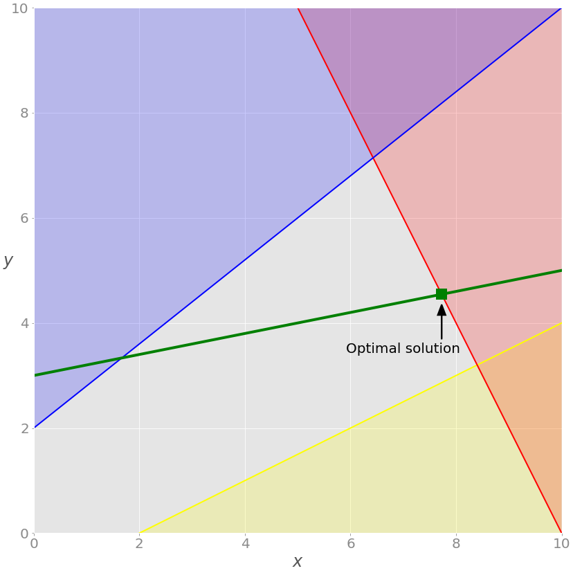
As discussed earlier, the optimal solutions to linear programming problems lie at the vertices of the feasible regions. In this case, the feasible region is just the portion of the green line between the blue and red lines. The optimal solution is the green square that represents the point of intersection between the green and red lines.
If you want to exclude the equality (green) constraint, just drop the parameters A_eq and b_eq from the linprog() call:
>>> opt = linprog(c=obj, A_ub=lhs_ineq, b_ub=rhs_ineq, bounds=bnd,
...               method="revised simplex")
>>> opt
     con: array([], dtype=float64)
     fun: -20.714285714285715
 message: 'Optimization terminated successfully.'
     nit: 2
   slack: array([0.        , 0.        , 9.85714286])
  status: 0
 success: True
       x: array([6.42857143, 7.14285714]))
The solution is different from the previous case. You can see it on the chart:
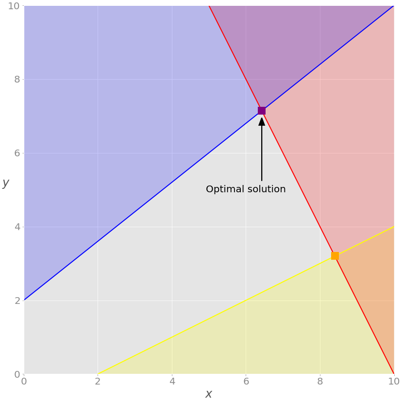
In this example, the optimal solution is the purple vertex of the feasible (gray) region where the red and blue constraints intersect. Other vertices, like the yellow one, have higher values for the objective function.
Example 2
You can use SciPy to solve the resource allocation problem stated in the earlier section:
As in the previous example, you need to extract the necessary vectors and matrix from the problem above, pass them as the arguments to .linprog(), and get the results:
>>> obj = [-20, -12, -40, -25]

>>> lhs_ineq = [[1, 1, 1, 1],  # Manpower
...             [3, 2, 1, 0],  # Material A
...             [0, 1, 2, 3]]  # Material B

>>> rhs_ineq = [ 50,  # Manpower
...             100,  # Material A
...              90]  # Material B

>>> opt = linprog(c=obj, A_ub=lhs_ineq, b_ub=rhs_ineq,
...               method="revised simplex")
>>> opt
     con: array([], dtype=float64)
     fun: -1900.0
 message: 'Optimization terminated successfully.'
     nit: 2
   slack: array([ 0., 40.,  0.])
  status: 0
 success: True
       x: array([ 5.,  0., 45.,  0.])
The result tells you that the maximal profit is 1900 and corresponds to x₁ = 5 and x₃ = 45. It’s not profitable to produce the second and fourth products under the given conditions. You can draw several interesting conclusions here:
-
The third product brings the largest profit per unit, so the factory will produce it the most.
-
The first slack is
0, which means that the values of the left and right sides of the manpower (first) constraint are the same. The factory produces50units per day, and that’s its full capacity. -
The second slack is
40because the factory consumes 60 units of raw material A (15 units for the first product plus 45 for the third) out of a potential100units. -
The third slack is
0, which means that the factory consumes all90units of the raw material B. This entire amount is consumed for the third product. That’s why the factory can’t produce the second or fourth product at all and can’t produce more than45units of the third product. It lacks the raw material B.
opt.status is 0 and opt.success is True, indicating that the optimization problem was successfully solved with the optimal feasible solution.
SciPy’s linear programming capabilities are useful mainly for smaller problems. For larger and more complex problems, you might find other libraries more suitable for the following reasons:
-
SciPy can’t run various external solvers.
-
SciPy can’t work with integer decision variables.
-
SciPy doesn’t provide classes or functions that facilitate model building. You have to define arrays and matrices, which might be a tedious and error-prone task for large problems.
-
SciPy doesn’t allow you to define maximization problems directly. You must convert them to minimization problems.
-
SciPy doesn’t allow you to define constraints using the greater-than-or-equal-to sign directly. You must use the less-than-or-equal-to instead.
Fortunately, the Python ecosystem offers several alternative solutions for linear programming that are very useful for larger problems. One of them is PuLP, which you’ll see in action in the next section.
Using PuLP
PuLP has a more convenient linear programming API than SciPy. You don’t have to mathematically modify your problem or use vectors and matrices. Everything is cleaner and less prone to errors.
As usual, you start by importing what you need:
from pulp import LpMaximize, LpProblem, LpStatus, lpSum, LpVariable
Now that you have PuLP imported, you can solve your problems.
Example 1
You’ll now solve this system with PuLP:
The first step is to initialize an instance of LpProblem to represent your model:
# Create the model
model = LpProblem(name="small-problem", sense=LpMaximize)
You use the sense parameter to choose whether to perform minimization (LpMinimize or 1, which is the default) or maximization (LpMaximize or -1). This choice will affect the result of your problem.
Once that you have the model, you can define the decision variables as instances of the LpVariable class:
# Initialize the decision variables
x = LpVariable(name="x", lowBound=0)
y = LpVariable(name="y", lowBound=0)
You need to provide a lower bound with lowBound=0 because the default value is negative infinity. The parameter upBound defines the upper bound, but you can omit it here because it defaults to positive infinity.
The optional parameter cat defines the category of a decision variable. If you’re working with continuous variables, then you can use the default value "Continuous".
You can use the variables x and y to create other PuLP objects that represent linear expressions and constraints:
>>> expression = 2 * x + 4 * y
>>> type(expression)
<class 'pulp.pulp.LpAffineExpression'>

>>> constraint = 2 * x + 4 * y >= 8
>>> type(constraint)
<class 'pulp.pulp.LpConstraint'>
When you multiply a decision variable with a scalar or build a linear combination of multiple decision variables, you get an instance of pulp.LpAffineExpression that represents a linear expression.
Note: You can add or subtract variables or expressions, and you can multiply them with constants because PuLP classes implement some of the Python special methods that emulate numeric types like __add__(), __sub__(), and __mul__(). These methods are used to customize the behavior of operators like +, -, and *.
Similarly, you can combine linear expressions, variables, and scalars with the operators ==, <=, or >= to get instances of pulp.LpConstraint that represent the linear constraints of your model.
Note: It’s also possible to build constraints with the rich comparison methods .__eq__(), .__le__(), and .__ge__() that define the behavior of the operators ==, <=, and >=.
Having this in mind, the next step is to create the constraints and objective function as well as to assign them to your model. You don’t need to create lists or matrices. Just write Python expressions and use the += operator to append them to the model:
# Add the constraints to the model
model += (2 * x + y <= 20, "red_constraint")
model += (4 * x - 5 * y >= -10, "blue_constraint")
model += (-x + 2 * y >= -2, "yellow_constraint")
model += (-x + 5 * y == 15, "green_constraint")
In the above code, you define tuples that hold the constraints and their names. LpProblem allows you to add constraints to a model by specifying them as tuples. The first element is a LpConstraint instance. The second element is a human-readable name for that constraint.
Setting the objective function is very similar:
# Add the objective function to the model
obj_func = x + 2 * y
model += obj_func
Alternatively, you can use a shorter notation:
# Add the objective function to the model
model += x + 2 * y
Now you have the objective function added and the model defined.
Note: You can append a constraint or objective to the model with the operator += because its class, LpProblem, implements the special method .__iadd__(), which is used to specify the behavior of +=.
For larger problems, it’s often more convenient to use lpSum() with a list or other sequence than to repeat the + operator. For example, you could add the objective function to the model with this statement:
# Add the objective function to the model
model += lpSum([x, 2 * y])
It produces the same result as the previous statement.
You can now see the full definition of this model:
>>> model
small-problem:
MAXIMIZE
1*x + 2*y + 0
SUBJECT TO
red_constraint: 2 x + y <= 20

blue_constraint: 4 x - 5 y >= -10

yellow_constraint: - x + 2 y >= -2

green_constraint: - x + 5 y = 15

VARIABLES
x Continuous
y Continuous
The string representation of the model contains all relevant data: the variables, constraints, objective, and their names.
Note: String representations are built by defining the special method .__repr__(). For more details about .__repr__(), check out Pythonic OOP String Conversion: __repr__ vs __str__ or When Should You Use .__repr__() vs .__str__() in Python?.
Finally, you’re ready to solve the problem. You can do that by calling .solve() on your model object. If you want to use the default solver (CBC), then you don’t need to pass any arguments:
# Solve the problem
status = model.solve()
.solve() calls the underlying solver, modifies the model object, and returns the integer status of the solution, which will be 1 if the optimum is found. For the rest of the status codes, see LpStatus[].
You can get the optimization results as the attributes of model. The function value() and the corresponding method .value() return the actual values of the attributes:
>>> print(f"status: {model.status}, {LpStatus[model.status]}")
status: 1, Optimal

>>> print(f"objective: {model.objective.value()}")
objective: 16.8181817

>>> for var in model.variables():
...     print(f"{var.name}: {var.value()}")
...
x: 7.7272727
y: 4.5454545

>>> for name, constraint in model.constraints.items():
...     print(f"{name}: {constraint.value()}")
...
red_constraint: -9.99999993922529e-08
blue_constraint: 18.181818300000003
yellow_constraint: 3.3636362999999996
green_constraint: -2.0000000233721948e-07)
model.objective holds the value of the objective function, model.constraints contains the values of the slack variables, and the objects x and y have the optimal values of the decision variables. model.variables() returns a list with the decision variables:
>>> model.variables()
[x, y]
>>> model.variables()[0] is x
True
>>> model.variables()[1] is y
True
As you can see, this list contains the exact objects that are created with the constructor of LpVariable.
The results are approximately the same as the ones you got with SciPy.
Note: Be careful with the method .solve()—it changes the state of the objects x and y!
You can see which solver was used by calling .solver:
>>> model.solver
<pulp.apis.coin_api.PULP_CBC_CMD object at 0x7f60aea19e50>
The output informs you that the solver is CBC. You didn’t specify a solver, so PuLP called the default one.
If you want to run a different solver, then you can specify it as an argument of .solve(). For example, if you want to use GLPK and already have it installed, then you can use solver=GLPK(msg=False) in the last line. Keep in mind that you’ll also need to import it:
from pulp import GLPK
Now that you have GLPK imported, you can use it inside .solve():
# Create the model
model = LpProblem(name="small-problem", sense=LpMaximize)

# Initialize the decision variables
x = LpVariable(name="x", lowBound=0)
y = LpVariable(name="y", lowBound=0)

# Add the constraints to the model
model += (2 * x + y <= 20, "red_constraint")
model += (4 * x - 5 * y >= -10, "blue_constraint")
model += (-x + 2 * y >= -2, "yellow_constraint")
model += (-x + 5 * y == 15, "green_constraint")

# Add the objective function to the model
model += lpSum([x, 2 * y])

# Solve the problem
status = model.solve(solver=GLPK(msg=False))
The msg parameter is used to display information from the solver. msg=False disables showing this information. If you want to include the information, then just omit msg or set msg=True.
Your model is defined and solved, so you can inspect the results the same way you did in the previous case:
>>> print(f"status: {model.status}, {LpStatus[model.status]}")
status: 1, Optimal

>>> print(f"objective: {model.objective.value()}")
objective: 16.81817

>>> for var in model.variables():
...     print(f"{var.name}: {var.value()}")
...
x: 7.72727
y: 4.54545

>>> for name, constraint in model.constraints.items():
...     print(f"{name}: {constraint.value()}")
...
red_constraint: -1.0000000000509601e-05
blue_constraint: 18.181830000000005
yellow_constraint: 3.3636299999999997
green_constraint: -2.000000000279556e-05
You got practically the same result with GLPK as you did with SciPy and CBC.
Let’s peek and see which solver was used this time:
>>> model.solver
<pulp.apis.glpk_api.GLPK_CMD object at 0x7f60aeb04d50>
As you defined above with the highlighted statement model.solve(solver=GLPK(msg=False)), the solver is GLPK.
You can also use PuLP to solve mixed-integer linear programming problems. To define an integer or binary variable, just pass cat="Integer" or cat="Binary" to LpVariable. Everything else remains the same:
# Create the model
model = LpProblem(name="small-problem", sense=LpMaximize)

# Initialize the decision variables: x is integer, y is continuous
x = LpVariable(name="x", lowBound=0, cat="Integer")
y = LpVariable(name="y", lowBound=0)

# Add the constraints to the model
model += (2 * x + y <= 20, "red_constraint")
model += (4 * x - 5 * y >= -10, "blue_constraint")
model += (-x + 2 * y >= -2, "yellow_constraint")
model += (-x + 5 * y == 15, "green_constraint")

# Add the objective function to the model
model += lpSum([x, 2 * y])

# Solve the problem
status = model.solve()
In this example, you have one integer variable and get different results from before:
>>> print(f"status: {model.status}, {LpStatus[model.status]}")
status: 1, Optimal

>>> print(f"objective: {model.objective.value()}")
objective: 15.8

>>> for var in model.variables():
...     print(f"{var.name}: {var.value()}")
...
x: 7.0
y: 4.4

>>> for name, constraint in model.constraints.items():
...     print(f"{name}: {constraint.value()}")
...
red_constraint: -1.5999999999999996
blue_constraint: 16.0
yellow_constraint: 3.8000000000000007
green_constraint: 0.0)

>>> model.solver
<pulp.apis.coin_api.PULP_CBC_CMD at 0x7f0f005c6210>
Now x is an integer, as specified in the model. (Technically it holds a float value with zero after the decimal point.) This fact changes the whole solution. Let’s show this on the graph:
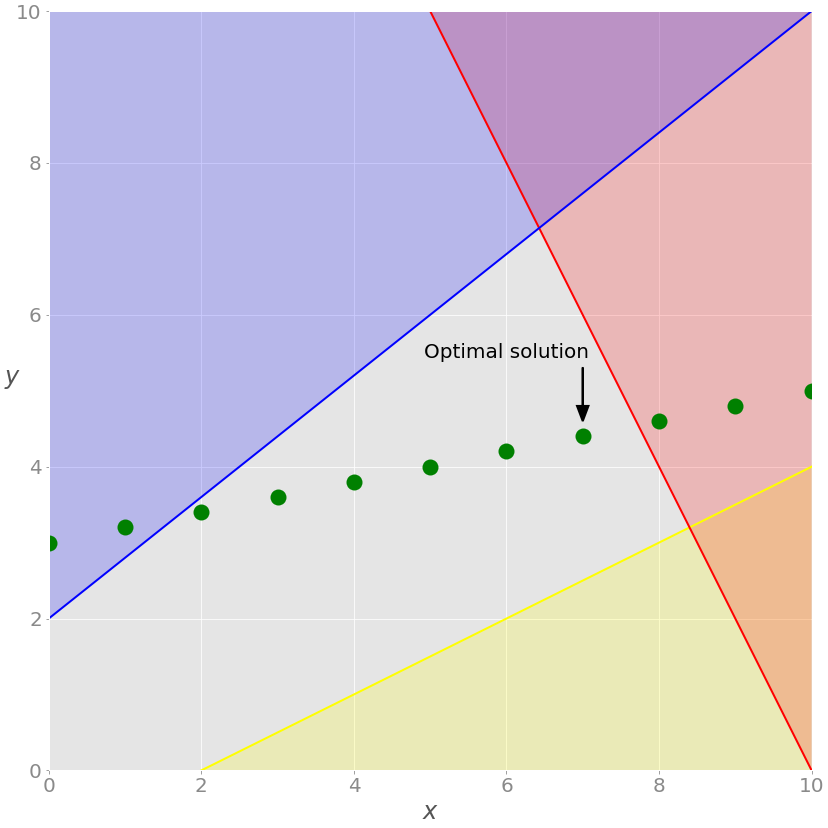
As you can see, the optimal solution is the rightmost green point on the gray background. This is the feasible solution with the largest values of both x and y, giving it the maximal objective function value.
GLPK is capable of solving such problems as well.
Example 2
Now you can use PuLP to solve the resource allocation problem from above:
The approach for defining and solving the problem is the same as in the previous example:
# Define the model
model = LpProblem(name="resource-allocation", sense=LpMaximize)

# Define the decision variables
x = {i: LpVariable(name=f"x{i}", lowBound=0) for i in range(1, 5)}

# Add constraints
model += (lpSum(x.values()) <= 50, "manpower")
model += (3 * x[1] + 2 * x[2] + x[3] <= 100, "material_a")
model += (x[2] + 2 * x[3] + 3 * x[4] <= 90, "material_b")

# Set the objective
model += 20 * x[1] + 12 * x[2] + 40 * x[3] + 25 * x[4]

# Solve the optimization problem
status = model.solve()

# Get the results
print(f"status: {model.status}, {LpStatus[model.status]}")
print(f"objective: {model.objective.value()}")

for var in x.values():
    print(f"{var.name}: {var.value()}")

for name, constraint in model.constraints.items():
    print(f"{name}: {constraint.value()}")
In this case, you use the dictionary x to store all decision variables. This approach is convenient because dictionaries can store the names or indices of decision variables as keys and the corresponding LpVariable objects as values. Lists or tuples of LpVariable instances can be useful as well.
The code above produces the following result:
status: 1, Optimal
objective: 1900.0
x1: 5.0
x2: 0.0
x3: 45.0
x4: 0.0
manpower: 0.0
material_a: -40.0
material_b: 0.0
As you can see, the solution is consistent with the one obtained using SciPy. The most profitable solution is to produce 5.0 units of the first product and 45.0 units of the third product per day.
Let’s make this problem more complicated and interesting. Say the factory can’t produce the first and third products in parallel due to a machinery issue. What’s the most profitable solution in this case?
Now you have another logical constraint: if x₁ is positive, then x₃ must be zero and vice versa. This is where binary decision variables are very useful. You’ll use two binary decision variables, y₁ and y₃, that’ll denote if the first or third products are generated at all:
 1model = LpProblem(name="resource-allocation", sense=LpMaximize)
 2
 3# Define the decision variables
 4x = {i: LpVariable(name=f"x{i}", lowBound=0) for i in range(1, 5)}
 5y = {i: LpVariable(name=f"y{i}", cat="Binary") for i in (1, 3)}
 6
 7# Add constraints
 8model += (lpSum(x.values()) <= 50, "manpower")
 9model += (3 * x[1] + 2 * x[2] + x[3] <= 100, "material_a")
10model += (x[2] + 2 * x[3] + 3 * x[4] <= 90, "material_b")
11
12M = 100
13model += (x[1] <= y[1] * M, "x1_constraint")
14model += (x[3] <= y[3] * M, "x3_constraint")
15model += (y[1] + y[3] <= 1, "y_constraint")
16
17# Set objective
18model += 20 * x[1] + 12 * x[2] + 40 * x[3] + 25 * x[4]
19
20# Solve the optimization problem
21status = model.solve()
22
23print(f"status: {model.status}, {LpStatus[model.status]}")
24print(f"objective: {model.objective.value()}")
25
26for var in model.variables():
27    print(f"{var.name}: {var.value()}")
28
29for name, constraint in model.constraints.items():
30    print(f"{name}: {constraint.value()}")
The code is very similar to the previous example except for the highlighted lines. Here are the differences:
-
Line 5 defines the binary decision variables
y[1]andy[3]held in the dictionaryy. -
Line 12 defines an arbitrarily large number
M. The value100is large enough in this case because you can’t have more than100units per day. -
Line 13 says that if
y[1]is zero, thenx[1]must be zero, else it can be any non-negative number. -
Line 14 says that if
y[3]is zero, thenx[3]must be zero, else it can be any non-negative number. -
Line 15 says that either
y[1]ory[3]is zero (or both are), so eitherx[1]orx[3]must be zero as well.
Here’s the solution:
status: 1, Optimal
objective: 1800.0
x1: 0.0
x2: 0.0
x3: 45.0
x4: 0.0
y1: 0.0
y3: 1.0
manpower: -5.0
material_a: -55.0
material_b: 0.0
x1_constraint: 0.0
x3_constraint: -55.0
y_constraint: 0.0
It turns out that the optimal approach is to exclude the first product and to produce only the third one.
Linear Programming Resources
Linear programming and mixed-integer linear programming are very important topics. If you want to learn more about them—and there’s much more to learn than what you saw here—then you can find plenty of resources. Here are a few to get started with:
- Wikipedia Linear Programming Article
- Wikipedia Integer Programming Article
- MIT Introduction to Mathematical Programming Course
- Brilliant.org Linear Programming Article
- CalcWorkshop What Is Linear Programming?
- BYJU’S Linear Programming Article
Gurobi Optimization is a company that offers a very fast commercial solver with a Python API. It also provides valuable resources on linear programming and mixed-integer linear programming, including the following:
- Linear Programming (LP) – A Primer on the Basics
- Mixed-Integer Programming (MIP) – A Primer on the Basics
- Tutorials
- Choosing a Math Programming Solver
If you’re in the mood to learn optimization theory, then there’s plenty of math books out there. Here are a few popular choices:
- Linear Programming: Foundations and Extensions
- Convex Optimization
- Model Building in Mathematical Programming
- Engineering Optimization: Theory and Practice
This is just a part of what’s available. Linear programming and mixed-integer linear programming are popular and widely used techniques, so you can find countless resources to help deepen your understanding.
Linear Programming Solvers
Just like there are many resources to help you learn linear programming and mixed-integer linear programming, there’s also a wide range of solvers that have Python wrappers available. Here’s a partial list:
Some of these libraries, like Gurobi, include their own Python wrappers. Others use external wrappers. For example, you saw that you can access CBC and GLPK with PuLP.
Conclusion
You now know what linear programming is and how to use Python to solve linear programming problems. You also learned that Python linear programming libraries are just wrappers around native solvers. When the solver finishes its job, the wrapper returns the solution status, the decision variable values, the slack variables, the objective function, and so on.
In this tutorial, you learned how to:
- Define a model that represents your problem
- Create a Python program for optimization
- Run the optimization program to find the solution to the problem
- Retrieve the result of optimization
You used SciPy with its own solver as well as PuLP with CBC and GLPK, but you also learned that there are many other linear programming solvers and Python wrappers. You’re now ready to dive into the world of linear programming!
If you have any questions or comments, then please put them in the comments section below.