Python has a design philosophy that stresses allowing programmers to express concepts readably and in fewer lines of code. This philosophy makes the language suitable for a diverse set of use cases: simple scripts for web, large web applications (like YouTube), scripting language for other platforms (like Blender and Autodesk’s Maya), and scientific applications in several areas, such as astronomy, meteorology, physics, and data science.
It is technically possible to implement scalar and matrix calculations using Python lists. However, this can be unwieldy, and performance is poor when compared to languages suited for numerical computation, such as MATLAB or Fortran, or even some general purpose languages, such as C or C++.
To circumvent this deficiency, several libraries have emerged that maintain Python’s ease of use while lending the ability to perform numerical calculations in an efficient manner. Two such libraries worth mentioning are NumPy (one of the pioneer libraries to bring efficient numerical computation to Python) and TensorFlow (a more recently rolled-out library focused more on deep learning algorithms).
- NumPy provides support for large multidimensional arrays and matrices along with a collection of mathematical functions to operate on these elements. The project relies on well-known packages implemented in other languages (like Fortran) to perform efficient computations, bringing the user both the expressiveness of Python and a performance similar to MATLAB or Fortran.
- TensorFlow is an open-source library for numerical computation originally developed by researchers and engineers working at the Google Brain team. The main focus of the library is to provide an easy-to-use API to implement practical machine learning algorithms and deploy them to run on CPUs, GPUs, or a cluster.
But how do these schemes compare? How much faster does the application run when implemented with NumPy instead of pure Python? What about TensorFlow? The purpose of this article is to begin to explore the improvements you can achieve by using these libraries.
To compare the performance of the three approaches, you’ll build a basic regression with native Python, NumPy, and TensorFlow.
Don’t miss the follow up tutorial: Click here to join the Real Python Newsletter and you’ll know when the next installment comes out.
Engineering the Test Data
To test the performance of the libraries, you’ll consider a simple two-parameter linear regression problem. The model has two parameters: an intercept term, w_0 and a single coefficient, w_1.
Given N pairs of inputs x and desired outputs d, the idea is to model the relationship between the outputs and the inputs using a linear model y = w_0 + w_1 * x where the output of the model y is approximately equal to the desired output d for every pair (x, d).
Technical Detail: The intercept term, w_0, is technically just a coefficient like w_1, but it can be interpreted as a coefficient that multiplies elements of a vector of 1s.
To generate the training set of the problem, use the following program:
import numpy as np

np.random.seed(444)

N = 10000
sigma = 0.1
noise = sigma * np.random.randn(N)
x = np.linspace(0, 2, N)
d = 3 + 2 * x + noise
d.shape = (N, 1)

# We need to prepend a column vector of 1s to `x`.
X = np.column_stack((np.ones(N, dtype=x.dtype), x))
print(X.shape)
(10000, 2)
This program creates a set of 10,000 inputs x linearly distributed over the interval from 0 to 2. It then creates a set of desired outputs d = 3 + 2 * x + noise, where noise is taken from a Gaussian (normal) distribution with zero mean and standard deviation sigma = 0.1.
By creating x and d in this way, you’re effectively stipulating that the optimal solution for w_0 and w_1 is 3 and 2, respectively.
Xplus = np.linalg.pinv(X)
w_opt = Xplus @ d
print(w_opt)
[[2.99536719]
 [2.00288672]]
There are several methods to estimate the parameters w_0 and w_1 to fit a linear model to the training set. One of the most-used is ordinary least squares, which is a well-known solution for the estimation of w_0 and w_1 in order to minimize the square of the error e, given by the summation of y - d for every training sample.
One way to easily compute the ordinary least squares solution is by using the Moore-Penrose pseudo-inverse of a matrix. This approach stems from the fact that you have X and d and are trying to solve for w_m, in the equation d = X @ w_m. (The @ symbol denotes matrix multiplication, which is supported by both NumPy and native Python as of PEP 465 and Python 3.5+.)
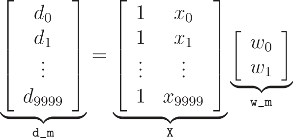
Using this approach, we can estimate w_m using w_opt = Xplus @ d, where Xplus is given by the pseudo-inverse of X, which can be calculated using numpy.linalg.pinv, resulting in w_0 = 2.9978 and w_1 = 2.0016, which is very close to the expected values of w_0 = 3 and w_1 = 2.
Note: Using w_opt = np.linalg.inv(X.T @ X) @ X.T @ d would yield the same solution. For more, see A Matrix Formulation of the Multiple Regression Model.
Although it is possible to use this deterministic approach to estimate the coefficients of the linear model, it is not possible for some other models, such as neural networks. In these cases, iterative algorithms are used to estimate a solution for the parameters of the model.
One of the most-used algorithms is gradient descent, which at a high level consists of updating the parameter coefficients until we converge on a minimized loss (or cost). That is, we have some cost function (often, the mean squared error—MSE), and we compute its gradient with respect to the network’s coefficients (in this case, the parameters w_0 and w_1), considering a step size mu. By performing this update many times (in many epochs), the coefficients converge to a solution that minimizes the cost function.
In the following sections, you’ll build and use gradient descent algorithms in pure Python, NumPy, and TensorFlow. To compare the performance of the three approaches, we’ll look at runtime comparisons on an Intel Core i7 4790K 4.0 GHz CPU.
Gradient Descent in Pure Python
Let’s start with a pure-Python approach as a baseline for comparison with the other approaches. The Python function below estimates the parameters w_0 and w_1 using gradient descent:
import itertools as it

def py_descent(x, d, mu, N_epochs):
    N = len(x)
    f = 2 / N

    # "Empty" predictions, errors, weights, gradients.
    y = [0] * N
    w = [0, 0]
    grad = [0, 0]

    for _ in it.repeat(None, N_epochs):
        # Can't use a generator because we need to
        # access its elements twice.
        err = tuple(i - j for i, j in zip(d, y))
        grad[0] = f * sum(err)
        grad[1] = f * sum(i * j for i, j in zip(err, x))
        w = [i + mu * j for i, j in zip(w, grad)]
        y = (w[0] + w[1] * i for i in x)
    return w
Above, everything is done with Python list comprehensions, slicing syntax, and the built-in sum() and zip() functions. Before running through each epoch, “empty” containers of zeros are initialized for y, w, and grad.
Technical Detail: py_descent above does use itertools.repeat() rather than for _ in range(N_epochs). The former is faster than the latter because repeat() does not need to manufacture a distinct integer for each loop. It just needs to update the reference count to None. The timeit module contains an example.
Now, use this to find a solution:
import time

x_list = x.tolist()
d_list = d.squeeze().tolist()  # Need 1d lists

# `mu` is a step size, or scaling factor.
mu = 0.001
N_epochs = 10000

t0 = time.time()
py_w = py_descent(x_list, d_list, mu, N_epochs)
t1 = time.time()

print(py_w)
[2.959859852416156, 2.0329649630002757]

print('Solve time: {:.2f} seconds'.format(round(t1 - t0, 2)))
Solve time: 18.65 seconds
With a step size of mu = 0.001 and 10,000 epochs, we can get a fairly precise estimate of w_0 and w_1. Inside the for loop, the gradients with respect to the parameters are calculated and used in turn to update the weights, moving in the opposite direction in order to minimize the MSE cost function.
At each epoch, after the update, the output of the model is calculated. The vector operations are performed using list comprehensions. We could have also updated y in-place, but that would not have been beneficial to performance.
The elapsed time of the algorithm is measured using the time library. It takes 18.65 seconds to estimate w_0 = 2.9598 and w_1 = 2.0329. While the timeit library can provide a more exact estimate of runtime by running multiple loops and disabling garbage collection, just viewing a single run with time suffices in this case, as you’ll see shortly.
Using NumPy
NumPy adds support for large multidimensional arrays and matrices along with a collection of mathematical functions to operate on them. The operations are optimized to run with blazing speed by relying on the projects BLAS and LAPACK for underlying implementation.
Using NumPy, consider the following program to estimate the parameters of the regression:
def np_descent(x, d, mu, N_epochs):
    d = d.squeeze()
    N = len(x)
    f = 2 / N

    y = np.zeros(N)
    err = np.zeros(N)
    w = np.zeros(2)
    grad = np.empty(2)

    for _ in it.repeat(None, N_epochs):
        np.subtract(d, y, out=err)
        grad[:] = f * np.sum(err), f * (err @ x)
        w = w + mu * grad
        y = w[0] + w[1] * x
    return w

np_w = np_descent(x, d, mu, N_epochs)
print(np_w)
[2.95985985 2.03296496]
The code block above takes advantage of vectorized operations with NumPy arrays (ndarrays). The only explicit for loop is the outer loop over which the training routine itself is repeated. List comprehensions are absent here because NumPy’s ndarray type overloads the arithmetic operators to perform array calculations in an optimized way.
You may notice there are a few alternate ways to go about solving this problem. For instance, you could use simply f * err @ X, where X is the 2d array that includes a column vector of ones, rather than our 1d x.
However, this is actually not all that efficient, because it requires a dot product of an entire column of ones with another vector (err), and we know that result will simply be np.sum(err). Similarly, w[0] + w[1] * x wastes less computation than w * X, in this specific case.
Let’s look at the timing comparison. As you’ll see below, the timeit module is needed here to get a more precise picture of runtime, as we’re now talking about fractions of a second rather than multiple seconds of runtime:
import timeit

setup = ("from __main__ import x, d, mu, N_epochs, np_descent;"
         "import numpy as np")
repeat = 5
number = 5  # Number of loops within each repeat

np_times = timeit.repeat('np_descent(x, d, mu, N_epochs)', setup=setup,
                         repeat=repeat, number=number)
timeit.repeat() returns a list. Each element is the total time taken to execute n loops of the statement. To get a single estimate of runtime, you can take the average time for a single call from the lower bound of the list of repeats:
print(min(np_times) / number)
0.31947448799983247
Using TensorFlow
TensorFlow is an open-source library for numerical computation originally developed by researchers and engineers working at the Google Brain team.
Using its Python API, TensorFlow’s routines are implemented as a graph of computations to perform. Nodes in the graph represent mathematical operations, and the graph edges represent the multidimensional data arrays (also called tensors) communicated between them.
At runtime, TensorFlow takes the graph of computations and runs it efficiently using optimized C++ code. By analyzing the graph of computations, TensorFlow is able to identify the operations that can be run in parallel. This architecture allows the use of a single API to deploy computation to one or more CPUs or GPUs in a desktop, server, or mobile device.
Using TensorFlow, consider the following program to estimate the parameters of the regression:
import tensorflow as tf

def tf_descent(X_tf, d_tf, mu, N_epochs):
    N = X_tf.get_shape().as_list()[0]
    f = 2 / N

    w = tf.Variable(tf.zeros((2, 1)), name="w_tf")
    y = tf.matmul(X_tf, w, name="y_tf")
    e = y - d_tf
    grad = f * tf.matmul(tf.transpose(X_tf), e)

    training_op = tf.assign(w, w - mu * grad)
    init = tf.global_variables_initializer()

    with tf.Session() as sess:
        init.run()
        for epoch in range(N_epochs):
            sess.run(training_op)
        opt = w.eval()
    return opt

X_tf = tf.constant(X, dtype=tf.float32, name="X_tf")
d_tf = tf.constant(d, dtype=tf.float32, name="d_tf")

tf_w = tf_descent(X_tf, d_tf, mu, N_epochs)
print(tf_w)
[[2.9598553]
 [2.032969 ]]
When you use TensorFlow, the data must be loaded into a special data type called a Tensor. Tensors mirror NumPy arrays in more ways than they are dissimilar.
type(X_tf)
<class 'tensorflow.python.framework.ops.Tensor'>
After the tensors are created from the training data, the graph of computations is defined:
- First, a variable tensor
wis used to store the regression parameters, which will be updated at each iteration. - Using
wandX_tf, the outputyis calculated using a matrix product, implemented withtf.matmul(). - The error is calculated and stored in the
etensor. - The gradients are computed, using the matrix approach, by multiplying the transpose of
X_tfby thee. - Finally, the update of the parameters of the regression is implemented with the
tf.assign()function. It creates a node that implements batch gradient descent, updating the next step tensorwtow - mu * grad.
It is worth noticing that the code until the training_op creation does not perform any computation. It just creates the graph of the computations to be performed. In fact, even the variables are not initialized yet. To perform the computations, it is necessary to create a session and use it to initialize the variables and run the algorithm to evaluate the parameters of the regression.
There are some different ways to initialize the variables and create the session to perform the computations. In this program, the line init = tf.global_variables_initializer() creates a node in the graph that will initialize the variables when it is run. The session is created in the with block, and init.run() is used to actually initialize the variables. Inside the with block, training_op is run for the desired number of epochs, evaluating the parameter of the regression, which have their final value stored in opt.
Here is the same code-timing structure that was used with the NumPy implementation:
setup = ("from __main__ import X_tf, d_tf, mu, N_epochs, tf_descent;"
         "import tensorflow as tf")

tf_times = timeit.repeat("tf_descent(X_tf, d_tf, mu, N_epochs)", setup=setup,
                         repeat=repeat, number=number)

print(min(tf_times) / number)
1.1982891103994917
It took 1.20 seconds to estimate w_0 = 2.9598553 and w_1 = 2.032969. It is worth noticing that the computation was performed on a CPU and the performance may be improved when run on a GPU.
Lastly, you could have also defined an MSE cost function and passed this to TensorFlow’s gradients() function, which performs automatic differentiation, finding the gradient vector of MSE with regard to the weights:
mse = tf.reduce_mean(tf.square(e), name="mse")
grad = tf.gradients(mse, w)[0]
However, the timing difference in this case is negligible.
Conclusion
The purpose of this article was to perform a preliminary comparison of the performance of a pure Python, a NumPy and a TensorFlow implementation of a simple iterative algorithm to estimate the coefficients of a linear regression problem.
The results for the elapsed time to run the algorithm are summarized in the table below:
| Implementation | Elapsed Time |
|---|---|
| Pure Python with list comprehensions | 18.65s |
| NumPy | 0.32s |
| TensorFlow on CPU | 1.20s |
While the NumPy and TensorFlow solutions are competitive (on CPU), the pure Python implementation is a distant third. While Python is a robust general-purpose programming language, its libraries targeted towards numerical computation will win out any day when it comes to large batch operations on arrays.
While the NumPy example proved quicker by a hair than TensorFlow in this case, it’s important to note that TensorFlow really shines for more complex cases. With our relatively elementary regression problem, using TensorFlow arguably amounts to “using a sledgehammer to crack a nut,” as the saying goes.
With TensorFlow, it is possible to build and train complex neural networks across hundreds or thousands of multi-GPU servers. In a future post, we will cover the setup to run this example in GPUs using TensorFlow and compare the results.
Get Notified: Don’t miss the follow up to this tutorial—Click here to join the Real Python Newsletter and you’ll know when the next installment comes out.
References
- The NumPy and TensorFlow home pages
- Aurélien Géron: Hands-On Machine Learning with Scikit-Learn and TensorFlow
- Look Ma, No
forLoops: Array Programming With NumPy - NumPy tutorials at Real Python
