
If you work with big data sets, you probably remember the “aha” moment along your Python journey when you discovered the pandas library. pandas is a game changer for data science and analytics, particularly if you came to Python because you were searching for something more powerful than Excel and VBA.
So what is it about pandas that has data scientists, analysts, and engineers like me raving? Well, the pandas documentation says that it uses:
“fast, flexible, and expressive data structures designed to make working with “relational” or “labeled” data both easy and intuitive.”
Fast, flexible, easy, and intuitive? That sounds great! If your job involves building complicated data models, you don’t want to spend half of your development hours waiting for modules to churn through big data sets. You want to dedicate your time and brainpower to interpreting your data, rather than painstakingly fumbling around with less powerful tools.
But I Heard That pandas Is Slow…
When I first started using pandas, I was advised that, while it was a great tool for dissecting data, pandas was too slow to use as a statistical modeling tool. Starting out, this proved true. I spent more than a few minutes twiddling my thumbs, waiting for pandas to churn through data.
But then I learned that pandas is built on top of the NumPy array structure, and so many of its operations are carried out in C, either via NumPy or through pandas’ own library of Python extension modules that are written in Cython and compiled to C. So, shouldn’t pandas be fast too?
It absolutely should be, if you use it the way it was intended!
The paradox is that what may otherwise “look like” Pythonic code can be suboptimal in pandas as far as efficiency is concerned. Like NumPy, pandas is designed for vectorized operations that operate on entire columns or datasets in one sweep. Thinking about each “cell” or row individually should generally be a last resort, not a first.
This Tutorial
To be clear, this is not a guide about how to over-optimize your pandas code. pandas is already built to run quickly if used correctly. Also, there’s a big difference between optimization and writing clean code.
This is a guide to using pandas Pythonically to get the most out of its powerful and easy-to-use built-in features. Additionally, you will learn a couple of practical time-saving tips, so you won’t be twiddling those thumbs every time you work with your data.
In this tutorial, you’ll cover the following:
- Advantages of using
datetimedata with time series - The most efficient route to doing batch calculations
- Saving time by storing data with HDFStore
To demonstrate these topics, I’ll take an example from my day job that looks at a time series of electricity consumption. After loading the data, you’ll successively progress through more efficient ways to get to the end result. One adage that holds true for most of pandas is that there is more than one way to get from A to B. This doesn’t mean, however, that all of the available options will scale equally well to larger, more demanding datasets.
Assuming that you already know how to do some basic data selection in pandas, let’s get started.
The Task at Hand
The goal of this example will be to apply time-of-use energy tariffs to find the total cost of energy consumption for one year. That is, at different hours of the day, the price for electricity varies, so the task is to multiply the electricity consumed for each hour by the correct price for the hour in which it was consumed.
Let’s read our data from a CSV file that has two columns: one for date plus time and one for electrical energy consumed in kilowatt hours (kWh):
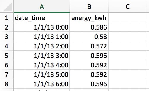
The rows contains the electricity used in each hour, so there are 365 x 24 = 8760 rows for the whole year. Each row indicates the usage for the “hour starting” at the time, so 1/1/13 0:00 indicates the usage for the first hour of January 1st.
Saving Time With Datetime Data
The first thing you need to do is to read your data from the CSV file with one of pandas’ I/O functions:
>>> import pandas as pd
>>> pd.__version__
'0.23.1'

# Make sure that `demand_profile.csv` is in your
# current working directory.
>>> df = pd.read_csv('demand_profile.csv')
>>> df.head()
     date_time  energy_kwh
0  1/1/13 0:00       0.586
1  1/1/13 1:00       0.580
2  1/1/13 2:00       0.572
3  1/1/13 3:00       0.596
4  1/1/13 4:00       0.592
This looks okay at first glance, but there’s a small issue. pandas and NumPy have a concept of dtypes (data types). If no arguments are specified, date_time will take on an object dtype:
>>> df.dtypes
date_time      object
energy_kwh    float64
dtype: object

>>> type(df.iat[0, 0])
str
This is not ideal. object is a container for not just str, but any column that can’t neatly fit into one data type. It would be arduous and inefficient to work with dates as strings. (It would also be memory-inefficient.)
For working with time series data, you’ll want the date_time column to be formatted as an array of datetime objects. (pandas calls this a Timestamp.) pandas makes each step here rather simple:
>>> df['date_time'] = pd.to_datetime(df['date_time'])
>>> df['date_time'].dtype
datetime64[ns]
(Note that you could alternatively use a pandas PeriodIndex in this case.)
You now have a DataFrame called df that looks much like our CSV file. It has two columns and a numerical index for referencing the rows.
>>> df.head()
               date_time    energy_kwh
0    2013-01-01 00:00:00         0.586
1    2013-01-01 01:00:00         0.580
2    2013-01-01 02:00:00         0.572
3    2013-01-01 03:00:00         0.596
4    2013-01-01 04:00:00         0.592
The code above is simple and easy, but how fast it? Let’s put it to the test using a timing decorator, which I have unoriginally called @timeit. This decorator largely mimics timeit.repeat() from Python’s standard library, but it allows you to return the result of the function itself and print its average runtime from multiple trials. (Python’s timeit.repeat() returns the timing results, not the function result.)
Creating a function and placing the @timeit decorator directly above it will mean that every time the function is called, it will be timed. The decorator runs an outer loop and an inner loop:
>>> @timeit(repeat=3, number=10)
... def convert(df, column_name):
...     return pd.to_datetime(df[column_name])

>>> # Read in again so that we have `object` dtype to start
>>> df['date_time'] = convert(df, 'date_time')
Best of 3 trials with 10 function calls per trial:
Function `convert` ran in average of 1.610 seconds.
The result? 1.6 seconds for 8760 rows of data. “Great,” you might say, “that’s no time at all.” But what if you encounter larger data sets—say, one year of electricity use at one-minute intervals? That’s 60 times more data, so you’ll end up waiting around one and a half minutes. That’s starting to sound less tolerable.
In actuality, I recently analyzed 10 years of hourly electricity data from 330 sites. Do you think I waited 88 minutes to convert datetimes? Absolutely not!
How can you speed this up? As a general rule, pandas will be far quicker the less it has to interpret your data. In this case, you will see huge speed improvements just by telling pandas what your time and date data looks like, using the format parameter. You can do this by using the strftime codes found here and entering them like this:
>>> @timeit(repeat=3, number=100)
>>> def convert_with_format(df, column_name):
...     return pd.to_datetime(df[column_name],
...                           format='%d/%m/%y %H:%M')
Best of 3 trials with 100 function calls per trial:
Function `convert_with_format` ran in average of 0.032 seconds.
The new result? 0.032 seconds, which is 50 times faster! So you’ve just saved about 86 minutes of processing time for my 330 sites. Not a bad improvement!
One finer detail is that the datetimes in the CSV are not in ISO 8601 format: you’d need YYYY-MM-DD HH:MM. If you don’t specify a format, pandas will use the dateutil package to convert each string to a date.
Conversely, if the raw datetime data is already in ISO 8601 format, pandas can immediately take a fast route to parsing the dates. This is one reason why being explicit about the format is so beneficial here. Another option is to pass infer_datetime_format=True parameter, but it generally pays to be explicit.
Note: pandas’ read_csv() also allows you to parse dates as a part of the file I/O step. See the parse_dates, infer_datetime_format, and date_parser parameters.
Simple Looping Over pandas Data
Now that your dates and times are in a convenient format, you are ready to get down to the business of calculating your electricity costs. Remember that cost varies by hour, so you will need to conditionally apply a cost factor to each hour of the day. In this example, the time-of-use costs will be defined as follows:
| Tariff Type | Cents per kWh | Time Range |
|---|---|---|
| Peak | 28 | 17:00 to 24:00 |
| Shoulder | 20 | 7:00 to 17:00 |
| Off-Peak | 12 | 0:00 to 7:00 |
If the price were a flat 28 cents per kWh for every hour of the day, most people familiar with pandas would know that this calculation could be achieved in one line:
>>> df['cost_cents'] = df['energy_kwh'] * 28
This will result in the creation of a new column with the cost of electricity for that hour:
               date_time    energy_kwh       cost_cents
0    2013-01-01 00:00:00         0.586           16.408
1    2013-01-01 01:00:00         0.580           16.240
2    2013-01-01 02:00:00         0.572           16.016
3    2013-01-01 03:00:00         0.596           16.688
4    2013-01-01 04:00:00         0.592           16.576
# ...
But our cost calculation is conditional on the time of day. This is where you will see a lot of people using pandas the way it was not intended: by writing a loop to do the conditional calculation.
For the rest of this tutorial, you’ll start from a less-than-ideal baseline solution and work up to a Pythonic solution that fully leverages pandas.
But what is Pythonic in the case of pandas? The irony is that it is those who are experienced in other (less user-friendly) coding languages such as C++ or Java that are particularly susceptible to this because they instinctively “think in loops.”
Let’s look at a loop approach that is not Pythonic and that many people take when they are unaware of how pandas is designed to be used. We will use @timeit again to see how fast this approach is.
First, let’s create a function to apply the appropriate tariff to a given hour:
def apply_tariff(kwh, hour):
    """Calculates cost of electricity for given hour."""
    if 0 <= hour < 7:
        rate = 12
    elif 7 <= hour < 17:
        rate = 20
    elif 17 <= hour < 24:
        rate = 28
    else:
        raise ValueError(f'Invalid hour: {hour}')
    return rate * kwh
Here’s the loop that isn’t Pythonic, in all its glory:
>>> # NOTE: Don't do this!
>>> @timeit(repeat=3, number=100)
... def apply_tariff_loop(df):
...     """Calculate costs in loop.  Modifies `df` inplace."""
...     energy_cost_list = []
...     for i in range(len(df)):
...         # Get electricity used and hour of day
...         energy_used = df.iloc[i]['energy_kwh']
...         hour = df.iloc[i]['date_time'].hour
...         energy_cost = apply_tariff(energy_used, hour)
...         energy_cost_list.append(energy_cost)
...     df['cost_cents'] = energy_cost_list
...
>>> apply_tariff_loop(df)
Best of 3 trials with 100 function calls per trial:
Function `apply_tariff_loop` ran in average of 3.152 seconds.
For people who picked up pandas after having written “pure Python” for some time prior, this design might seem natural: you have a typical “for each x, conditional on y, do z.”
However, this loop is clunky. You can consider the above to be an “antipattern” in pandas for several reasons. Firstly, it needs to initialize a list in which the outputs will be recorded.
Secondly, it uses the opaque object range(0, len(df)) to loop over, and then after applying apply_tariff(), it has to append the result to a list that is used to make the new DataFrame column. It also does what is called chained indexing with df.iloc[i]['date_time'], which often leads to unintended results.
But the biggest issue with this approach is the time cost of the calculations. On my machine, this loop took over 3 seconds for 8760 rows of data. Next, you’ll look at some improved solutions for iteration over pandas structures.
Looping with .itertuples() and .iterrows()
What other approaches can you take? Well, pandas has actually made the for i in range(len(df)) syntax redundant by introducing the DataFrame.itertuples() and DataFrame.iterrows() methods. These are both generator methods that yield one row at a time.
.itertuples() yields a namedtuple for each row, with the row’s index value as the first element of the tuple. A nametuple is a data structure from Python’s collections module that behaves like a Python tuple but has fields accessible by attribute lookup.
.iterrows() yields pairs (tuples) of (index, Series) for each row in the DataFrame.
While .itertuples() tends to be a bit faster, let’s stay in pandas and use .iterrows() in this example, because some readers might not have run across nametuple. Let’s see what this achieves:
>>> @timeit(repeat=3, number=100)
... def apply_tariff_iterrows(df):
...     energy_cost_list = []
...     for index, row in df.iterrows():
...         # Get electricity used and hour of day
...         energy_used = row['energy_kwh']
...         hour = row['date_time'].hour
...         # Append cost list
...         energy_cost = apply_tariff(energy_used, hour)
...         energy_cost_list.append(energy_cost)
...     df['cost_cents'] = energy_cost_list
...
>>> apply_tariff_iterrows(df)
Best of 3 trials with 100 function calls per trial:
Function `apply_tariff_iterrows` ran in average of 0.713 seconds.
Some marginal gains have been made. The syntax is more explicit, and there is less clutter in your row value references, so it’s more readable. In terms of time gains, is almost 5 five times quicker!
However, there is more room for improvement. You’re still using some form of a Python for loop, meaning that each and every function call is done in Python when it could ideally be done in a faster language built into pandas’ internal architecture.
pandas’ .apply()
You can further improve this operation using the .apply() method instead of .iterrows(). pandas’ .apply() method takes functions (callables) and applies them along an axis of a DataFrame (all rows, or all columns). In this example, a lambda function will help you pass the two columns of data into apply_tariff():
>>> @timeit(repeat=3, number=100)
... def apply_tariff_withapply(df):
...     df['cost_cents'] = df.apply(
...         lambda row: apply_tariff(
...             kwh=row['energy_kwh'],
...             hour=row['date_time'].hour),
...         axis=1)
...
>>> apply_tariff_withapply(df)
Best of 3 trials with 100 function calls per trial:
Function `apply_tariff_withapply` ran in average of 0.272 seconds.
The syntactic advantages of .apply() are clear, with a significant reduction in the number of lines and very readable, explicit code. In this case, the time taken was roughly half that of the .iterrows() method.
However, this is not yet “blazingly fast.” One reason is that .apply() will try internally to loop over Cython iterators. But in this case, the lambda that you passed isn’t something that can be handled in Cython, so it’s called in Python, which is consequently not all that fast.
If you were to use .apply() for my 10 years of hourly data for 330 sites, you’d be looking at around 15 minutes of processing time. If this calculation were intended to be a small part of a larger model, you’d really want to speed things up. That’s where vectorized operations come in handy.
Selecting Data With .isin()
Earlier, you saw that if there were a single electricity price, you could apply that price across all the electricity consumption data in one line of code (df['energy_kwh'] * 28). This particular operation was an example of a vectorized operation, and it is the fastest way to do things in pandas.
But how can you apply condition calculations as vectorized operations in pandas? One trick is to select and group parts the DataFrame based on your conditions and then apply a vectorized operation to each selected group.
In this next example, you will see how to select rows with pandas’ .isin() method and then apply the appropriate tariff in a vectorized operation. Before you do this, it will make things a little more convenient if you set the date_time column as the DataFrame’s index:
df.set_index('date_time', inplace=True)

@timeit(repeat=3, number=100)
def apply_tariff_isin(df):
    # Define hour range Boolean arrays
    peak_hours = df.index.hour.isin(range(17, 24))
    shoulder_hours = df.index.hour.isin(range(7, 17))
    off_peak_hours = df.index.hour.isin(range(0, 7))

    # Apply tariffs to hour ranges
    df.loc[peak_hours, 'cost_cents'] = df.loc[peak_hours, 'energy_kwh'] * 28
    df.loc[shoulder_hours,'cost_cents'] = df.loc[shoulder_hours, 'energy_kwh'] * 20
    df.loc[off_peak_hours,'cost_cents'] = df.loc[off_peak_hours, 'energy_kwh'] * 12
Let’s see how this compares:
>>> apply_tariff_isin(df)
Best of 3 trials with 100 function calls per trial:
Function `apply_tariff_isin` ran in average of 0.010 seconds.
To understand what’s happening in this code, you need to know that the .isin() method is returning an array of Boolean values that looks like this:
[False, False, False, ..., True, True, True]
These values identify which DataFrame indices (datetimes) fall within the hour range specified. Then, when you pass these Boolean arrays to the DataFrame’s .loc indexer, you get a slice of the DataFrame that only includes rows that match those hours. After that, it is simply a matter of multiplying the slice by the appropriate tariff, which is a speedy vectorized operation.
How does this compare to our looping operations above? Firstly, you may notice that you no longer need apply_tariff(), because all the conditional logic is applied in the selection of the rows. So there is a huge reduction in the lines of code you have to write and in the Python code that is called.
What about the processing time? 315 times faster than the loop that wasn’t Pythonic, around 71 times faster than .iterrows() and 27 times faster that .apply(). Now you are moving at the kind of speed you need to get through big data sets nice and quickly.
Can We Do Better?
In apply_tariff_isin(), we are still admittedly doing some “manual work” by calling df.loc and df.index.hour.isin() three times each. You could argue that this solution isn’t scalable if we had a more granular range of time slots. (A different rate for each hour would require 24 .isin() calls.) Luckily, you can do things even more programmatically with pandas’ pd.cut() function in this case:
@timeit(repeat=3, number=100)
def apply_tariff_cut(df):
    cents_per_kwh = pd.cut(x=df.index.hour,
                           bins=[0, 7, 17, 24],
                           include_lowest=True,
                           labels=[12, 20, 28]).astype(int)
    df['cost_cents'] = cents_per_kwh * df['energy_kwh']
Let’s take a second to see what’s going on here. pd.cut() is applying an array of labels (our costs) according to which bin each hour belongs in. Note that the include_lowest parameter indicates whether the first interval should be left-inclusive or not. (You want to include time=0 in a group.)
This is a fully vectorized way to get to your intended result, and it comes out on top in terms of timing:
>>> apply_tariff_cut(df)
Best of 3 trials with 100 function calls per trial:
Function `apply_tariff_cut` ran in average of 0.003 seconds.
So far, you’ve built up from taking potentially over an hour to under a second to process the full 300-site dataset. Not bad! There is one last option, though, which is to use NumPy functions to manipulate the underlying NumPy arrays for each DataFrame, and then to integrate the results back into pandas data structures.
Don’t Forget NumPy!
One point that should not be forgotten when you are using pandas is that pandas Series and DataFrames are designed on top of the NumPy library. This gives you even more computation flexibility, because pandas works seamlessly with NumPy arrays and operations.
In this next case you’ll use NumPy’s digitize() function. It is similar to pandas’ cut() in that the data will be binned, but this time it will be represented by an array of indexes representing which bin each hour belongs to. These indexes are then applied to a prices array:
@timeit(repeat=3, number=100)
def apply_tariff_digitize(df):
    prices = np.array([12, 20, 28])
    bins = np.digitize(df.index.hour.values, bins=[7, 17, 24])
    df['cost_cents'] = prices[bins] * df['energy_kwh'].values
Like the cut() function, this syntax is wonderfully concise and easy to read. But how does it compare in speed? Let’s see:
>>> apply_tariff_digitize(df)
Best of 3 trials with 100 function calls per trial:
Function `apply_tariff_digitize` ran in average of 0.002 seconds.
At this point, there’s still a performance improvement, but it’s becoming more marginal in nature. This is probably a good time to call it a day on hacking away at code improvement and think about the bigger picture.
With pandas, it can help to maintain “hierarchy,” if you will, of preferred options for doing batch calculations like you’ve done here. These will usually rank from fastest to slowest (and most to least flexible):
- Use vectorized operations: pandas methods and functions with no
forloops. - Use the
.apply()method with a callable. - Use
.itertuples(): iterate over DataFrame rows asnamedtuplesfrom Python’scollectionsmodule. - Use
.iterrows(): iterate over DataFrame rows as (index,pd.Series) pairs. While a pandas Series is a flexible data structure, it can be costly to construct each row into a Series and then access it. - Use “element-by-element” for loops, updating each cell or row one at a time with
df.locordf.iloc. (Or,.at/.iatfor fast scalar access.)
Don’t Take My Word For It: The order of precedence above is a suggestion straight from a core pandas developer.
You can learn more about your options in How to Iterate Over Rows in pandas, and Why You Shouldn’t.
Here’s the “order of precedence” above at work, with each function you’ve built here:
| Function | Runtime (seconds) |
|---|---|
apply_tariff_loop() |
3.152 |
apply_tariff_iterrows() |
0.713 |
apply_tariff_withapply() |
0.272 |
apply_tariff_isin() |
0.010 |
apply_tariff_cut() |
0.003 |
apply_tariff_digitize() |
0.002 |
Prevent Reprocessing with HDFStore
Now that you have looked at quick data processes in pandas, let’s explore how to avoid reprocessing time altogether with HDFStore, which was recently integrated into pandas.
Often when you are building a complex data model, it is convenient to do some pre-processing of your data. For example, if you had 10 years of minute-frequency electricity consumption data, simply converting the date and time to datetime might take 20 minutes, even if you specify the format parameter. You really only want to have to do this once, not every time you run your model, for testing or analysis.
A very useful thing you can do here is pre-process and then store your data in its processed form to be used when needed. But how can you store data in the right format without having to reprocess it again? If you were to save as CSV, you would simply lose your datetime objects and have to re-process it when accessing again.
pandas has a built-in solution for this which uses HDF5 , a high-performance storage format designed specifically for storing tabular arrays of data. Pandas’ HDFStore class allows you to store your DataFrame in an HDF5 file so that it can be accessed efficiently, while still retaining column types and other metadata. It is a dictionary-like class, so you can read and write just as you would for a Python dict object.
Here’s how you would go about storing your pre-processed electricity consumption DataFrame, df, in an HDF5 file:
# Create storage object with filename `processed_data`
data_store = pd.HDFStore('processed_data.h5')

# Put DataFrame into the object setting the key as 'preprocessed_df'
data_store['preprocessed_df'] = df
data_store.close()
Now you can shut your computer down and take a break knowing that you can come back and your processed data will be waiting for you when you need it. No reprocessing required. Here’s how you would access your data from the HDF5 file, with data types preserved:
# Access data store
data_store = pd.HDFStore('processed_data.h5')

# Retrieve data using key
preprocessed_df = data_store['preprocessed_df']
data_store.close()
A data store can house multiple tables, with the name of each as a key.
Just a note about using the HDFStore in pandas: you will need to have PyTables >= 3.0.0 installed, so after you have installed pandas, make sure to update PyTables like this:
pip install --upgrade tables
Conclusions
If you don’t feel like your pandas project is fast, flexible, easy, and intuitive, consider rethinking how you’re using the library.
The examples you’ve explored here are fairly straightforward but illustrate how the proper application of pandas features can make vast improvements to runtime and code readability to boot. Here are a few rules of thumb that you can apply next time you’re working with large data sets in pandas:
-
Try to use vectorized operations where possible rather than approaching problems with the
for x in df...mentality. If your code is home to a lot offorloops, it might be better suited to working with native Python data structures, because pandas otherwise comes with a lot of overhead. -
If you have more complex operations where vectorization is simply impossible or too difficult to work out efficiently, use the
.apply()method. -
If you do have to loop over your array (which does happen), use
.iterrows()or.itertuples()to improve speed and syntax. -
pandas has a lot of optionality, and there are almost always several ways to get from A to B. Be mindful of this, compare how different routes perform, and choose the one that works best in the context of your project.
-
Once you’ve got a data cleaning script built, avoid reprocessing by storing your intermediate results with HDFStore.
-
Integrating NumPy into pandas operations can often improve speed and simplify syntax.