Probability distributions describe the likelihood of all possible outcomes of an event or experiment. The normal distribution is one of the most useful probability distributions because it models many natural phenomena very well. With NumPy, you can create random number samples from the normal distribution.
This distribution is also called the Gaussian distribution or simply the bell curve. The latter hints at the shape of the distribution when you plot it:
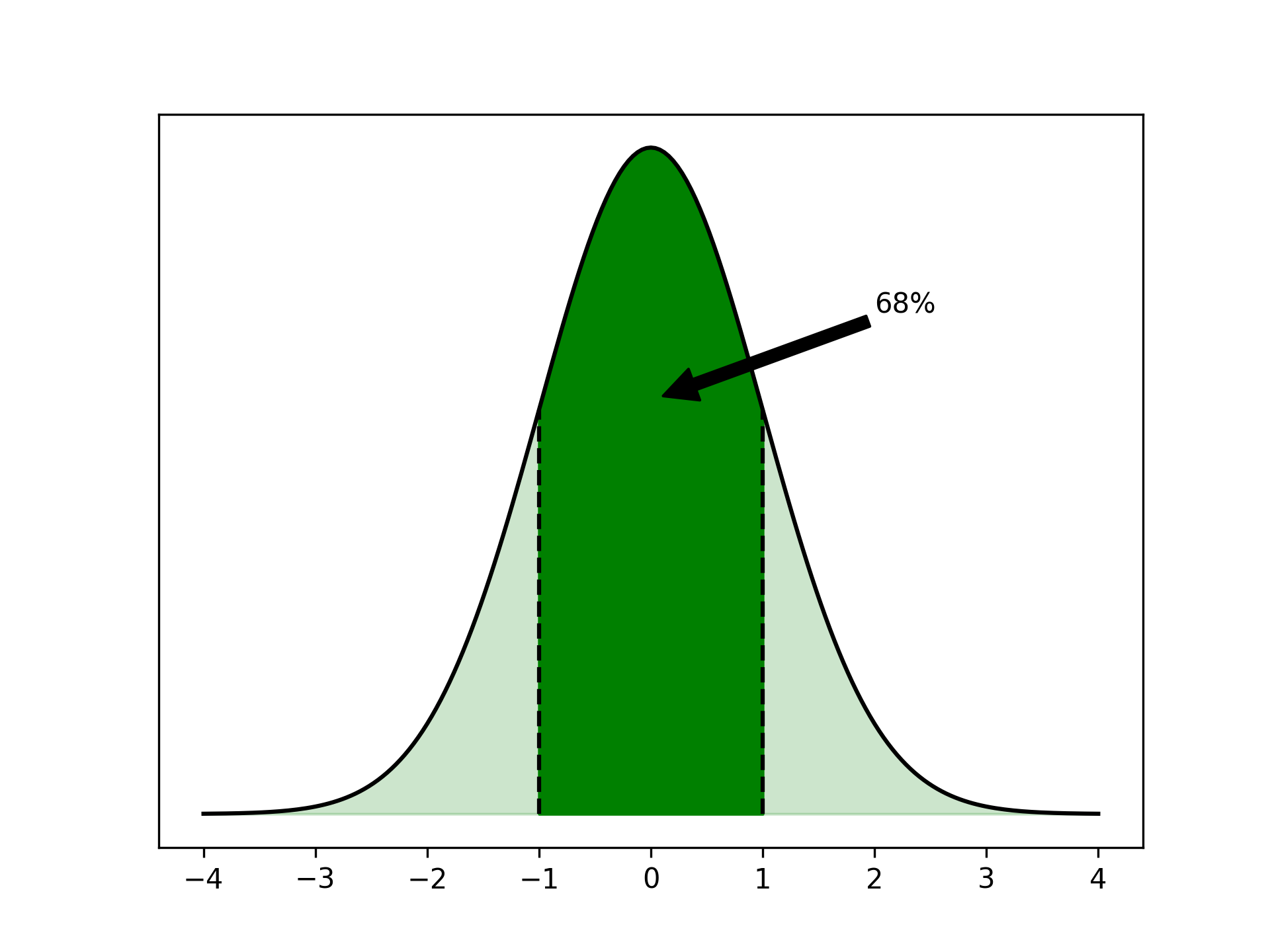
The normal distribution is symmetrical around its peak. Because of this symmetry, the mean of the distribution, often denoted by μ, is at that peak. The standard deviation, σ, describes how spread out the distribution is.
If some samples are normally distributed, then it’s probable that a random sample has a value close to the mean. In fact, about 68 percent of all samples are within one standard deviation of the mean.
You can interpret the area under the curve in the plot as a measure of probability. The darkly colored area, which represents all samples less than one standard deviation from the mean, is 68 percent of the full area under the curve.
In this tutorial, you’ll learn how you can use Python’s NumPy library to work with the normal distribution, and in particular how to create random numbers that are normally distributed. Along the way, you’ll get to know NumPy’s random number generator (RNG) and how to ensure that you can work with randomness in a reproducible manner.
You’ll also see how to visualize probability distributions with Matplotlib and histograms, as well as the effect of manipulating the mean and standard deviation. The central limit theorem explains the importance of the normal distribution. It describes how the average for any repeated experiment or measurement approximates the normal distribution.
As you’ll learn, you can do some powerful statistical analysis with the right Python code. To get the code from this tutorial, click the link below:
Free Bonus: Click here to download the free sample code that you’ll use to generate random numbers from a normal distribution in NumPy.
To follow along, you’ll need to install a few packages. First, create and activate a virtual environment. Then run the following pip command:
$ python -m pip install numpy matplotlib scipy
In addition to grabbing NumPy, you’ve installed Matplotlib and SciPy, so you’re ready to roll.
How to Use NumPy to Generate Normally Distributed Random Numbers
NumPy includes a full subpackage, numpy.random, dedicated to working with random numbers. For historical reasons, this package includes many functions. However, you should usually start by instantiating a default random number generator (RNG):
>>> import numpy as np
>>> rng = np.random.default_rng()
>>> rng
Generator(PCG64) at 0x7F00828DD8C0
The RNG can generate random numbers from many different distributions. To sample from the normal distribution, you’ll use .normal():
>>> rng.normal()
0.7630063999485851

>>> rng.normal()
0.46664545470659285

>>> rng.normal()
0.18800887515990947
While these numbers look random, whatever that means, it’s hard to confirm that one or a few numbers are drawn from a given distribution. You can ask NumPy to draw many numbers at once:
>>> numbers = rng.normal(size=10_000)

>>> numbers.mean()
0.004567244040854705

>>> numbers.std()
1.0058207076330512
Here you generate ten thousand normally distributed numbers. If you don’t specify any other parameters, then NumPy will create so-called standard normally distributed numbers that are centered around μ = 0 and have a standard deviation σ = 1. You confirm that the mean of your numbers is approximately zero. You also use .std() to check that the standard deviation is close to one.
NumPy can work with multidimensional arrays of numbers. You can specify size using a tuple to create N-dimensional arrays:
>>> rng.normal(size=(2, 4))
array([[ 0.44284801, -0.5197292 ,  0.36472606, -0.21618958],
       [-0.45235572,  0.04395177, -0.09295108, -0.70332948]])
In this case, you created a two-dimensional array of normally distributed random numbers with two rows and four columns. Organizing random data in several dimensions can be useful if you’re modeling repeated experiments. You’ll see a practical example of this later.
Plot Your Normally Distributed Numbers
When you’re modeling, looking at one single outcome usually isn’t that interesting. Instead, you want to look at many samples and try to get an idea of their distribution. For these kinds of overviews, visualizing a distribution by plotting a histogram of your numbers is powerful.
For the first example, use the numbers that you created above:
>>> import numpy as np
>>> rng = np.random.default_rng()
>>> numbers = rng.normal(size=10_000)
You can plot the ten thousand numbers in a histogram:
>>> import matplotlib.pyplot as plt
>>> plt.hist(numbers)
>>> plt.show()
Running plt.show() will show the histogram in a separate window. It’ll look something like this:
In a histogram, your values are grouped together in so-called bins. Above, you can count the blue bars to see that the histogram has ten bins. Note that the outermost bars are small and hard to spot.
The vertical axis of the histogram shows how many samples fall into each bin. The shape of the histogram shows some of the characteristics that you’d associate with the normal distribution. It’s symmetrical, has one clearly defined peak, and tapers off to the sides.
Depending on the number of samples in your dataset, you may want to increase the number of bins in your visualization. You can do this by specifying bins:
>>> plt.hist(numbers, bins=100)
>>> plt.show()
By increasing the number of bins to 100, you’ll get a smoother histogram:

Your choice of number of bins may change the look of the histogram slightly, so you should try a few different choices when you’re exploring your data.
Note that when you have more bins, there’ll be fewer values in each bin. This means that the absolute numbers on your y-axis are rarely interesting. They’ll scale based on the number of observations and the number of bins. For example, you can see that the counts in your first plot are about ten times higher than in the second one, where you use ten times as many bins.
You can calculate the area of the histogram by multiplying the number of observations with the width of a bin. The width of a single bin depends on the minimum and maximum observations and the number of bins. For the histogram with 100 bins, you’ll get the following:
>>> bins = 100
>>> bin_width = (numbers.max() - numbers.min()) / bins
>>> hist_area = len(numbers) * bin_width
>>> hist_area
763.8533882079863
Again, this value usually isn’t very interesting on its own. However, it can be useful if you want to compare your histogram with a theoretical normal distribution.
The SciPy library contains several functions named pdf(). These are probability density functions. You can use these to plot theoretical probability distributions:
>>> import scipy.stats
>>> x = np.linspace(-4, 4, 101)
>>> plt.plot(x, scipy.stats.norm.pdf(x))
>>> plt.show()
Here, you use scipy.stats.norm.pdf() to calculate the normal distribution for values of x between -4 and 4. This creates the following plot:
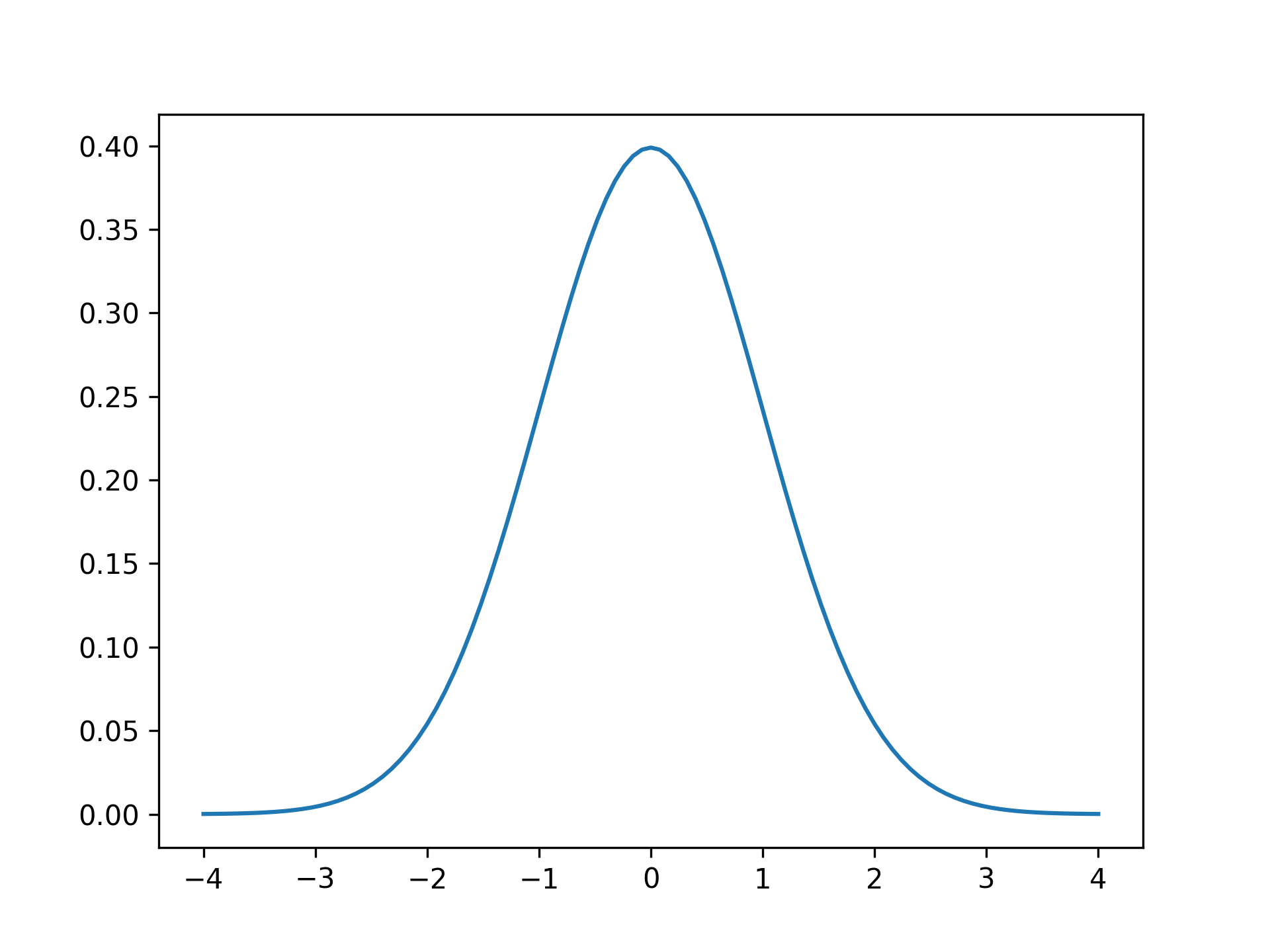
You can recognize the symmetrical curve with a single peak. By definition, the area under the curve of a probability density function is one. Therefore, if you want to compare your histogram of observations with the theoretical curve, then you need to scale the latter:
>>> x = np.linspace(numbers.min(), numbers.max(), 101)
>>> plt.hist(numbers, bins=100)
>>> plt.plot(x, scipy.stats.norm.pdf(x) * hist_area)
>>> plt.show()
Here, you scale the probability density function by the area of the histogram, which you calculated earlier. The resulting plot shows the normal distribution overlayed on top of the histogram:
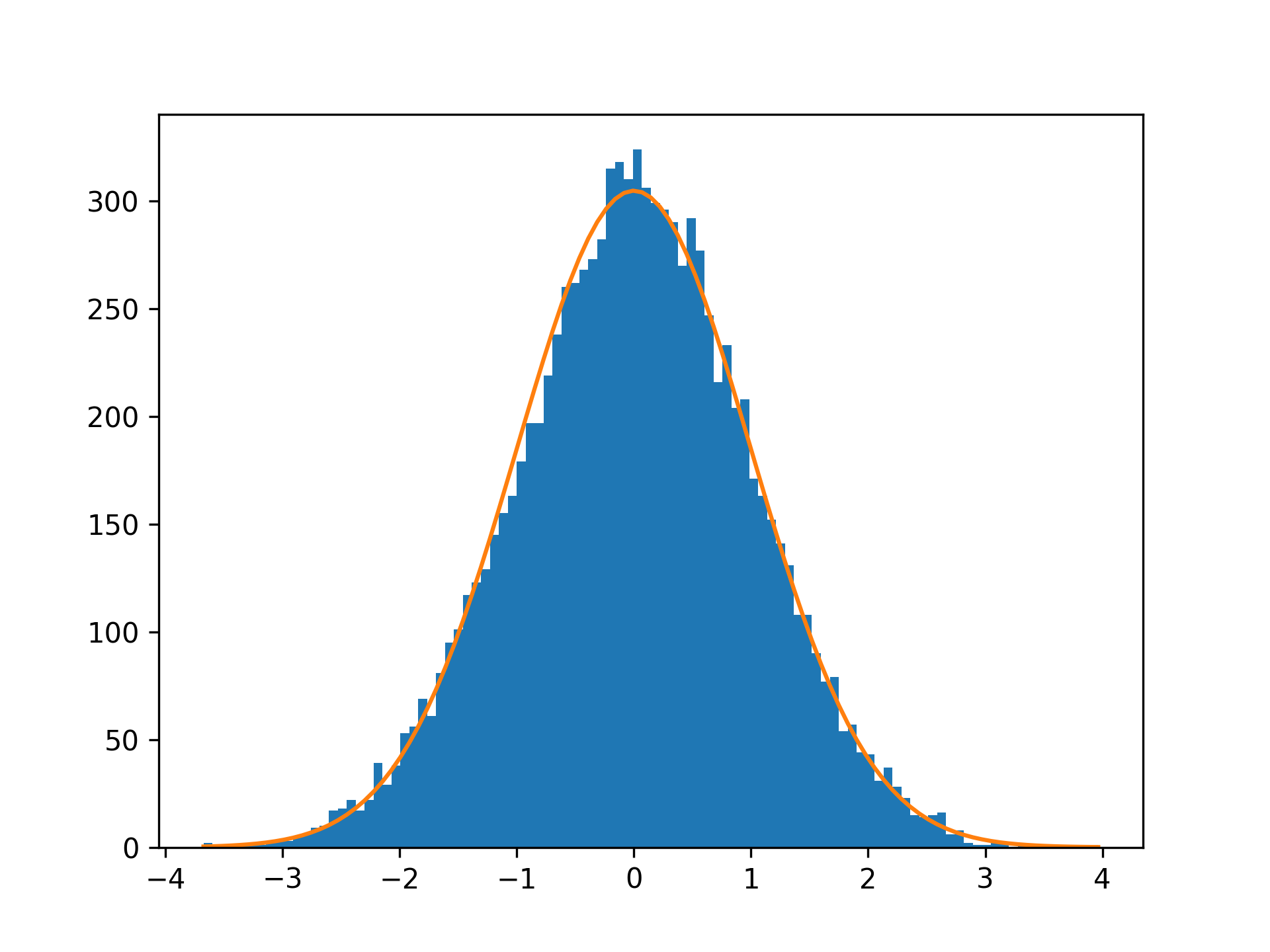
By visual inspection, you can see that your random data follow the normal distribution fairly well.
So far, you’ve seen how you can work with the normal distribution in NumPy. In the next sections, you’ll learn more about how and why the normal distribution is useful.
Specify the Mean and Standard Deviation
There are many examples of naturally occuring data that are normally distributed, including birth weights, adult heights, and shoe sizes. Say that you want to model a machine that packs bags of wheat. Through observation and measurements, you learn that the weight of wheat in each bag is normally distributed with a mean of μ = 1023 grams and a standard deviation of σ = 19 grams.
Previously, you’ve seen normal distributions that have been centered around μ = 0. However, you can define the normal distribution with any mean, μ, and any positive standard deviation, σ. In NumPy, you do this by specifying two parameters:
>>> import numpy as np
>>> rng = np.random.default_rng()
>>> weights = rng.normal(1023, 19, size=5_000)
>>> weights[:3]
array([1037.4971216 , 1031.86626364, 1026.57216863])
In contrast to earlier, now your random values are mostly just above 1000. You can calculate the mean and standard deviation of your observations:
>>> weights.mean()
1023.3071473510166

>>> weights.std()
19.25233332725017
Again, the characteristics of your random numbers are close to their theoretical values but not exactly equal. You can plot your data:
>>> import matplotlib.pyplot as plt
>>> plt.hist(weights, bins=50)
>>> plt.show()
These commands produce a plot like the following:
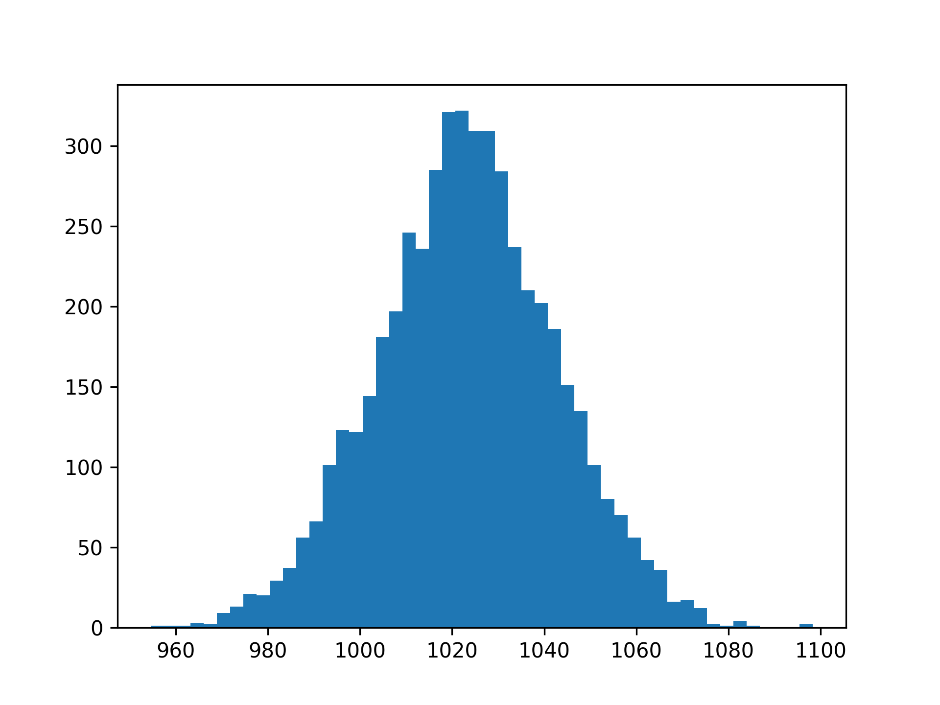
While you recognize the shape of the histogram, note that the x-axis is shifted so that most values are above 1000. Indeed, you can use NumPy to calculate the ratio of observations that are below 1000 grams:
>>> np.mean(weights < 1000)
0.117
NumPy calculates a Boolean expression like weights < 1000 element-wise. The result is an array of True and False values depending on the weight of each bag of wheat. Because True and False can be interpreted as 1 and 0, respectively, you can use mean() to calculate the ratio of True values.
In the example above, you see that 11.7 percent of the bags have a measured weight that’s less than 1000 grams. You can also estimate a similar number by looking at your plot. The area under the curve to the left of x = 1000 represents the lighter wheat bags.
You’ve seen that you can generate normal numbers with a given mean and standard deviation. In the next section, you’ll look more closely at NumPy’s random number generator.
Work With Random Numbers in NumPy
Creating random numbers in a deterministic system like a computer isn’t trivial. Most random number generators don’t produce true randomness. Instead, they generate numbers through a deterministic and reproducible process such that the numbers appear to be random.
In general terms, a random number generator—or more accurately, a pseudo-random number generator (PRNG)—is an algorithm that starts from a known seed and generates a pseudo-random number from it. One advantage of such a generator is that you can reproduce the random numbers:
>>> import numpy as np

>>> rng = np.random.default_rng(seed=2310)
>>> rng.normal(size=3)
array([0.7630064 , 0.46664545, 0.18800888])

>>> rng = np.random.default_rng(seed=2310)
>>> rng.normal(size=3)
array([0.7630064 , 0.46664545, 0.18800888])

>>> rng = np.random.default_rng(seed=2801)
>>> rng.normal(size=3)
array([-1.90550297,  0.05608914, -0.29362926])
If you create the random number generator with a specific seed, then you can re-create the same random numbers later by using the same seed. In this example, the second call to .normal() generates the same numbers as the first one. If, on the other hand, you initialize the generator with a different seed, then you get different random numbers.
Historically, you didn’t use an explicit random number generator when working with random numbers in NumPy. Instead, you called functions like np.random.normal() directly. However, NumPy 1.17 introduced explicit random number generators, and you’re encouraged to use this new way of working with random numbers as much as possible.
One advantage of the new machinery is that it’s more transparent. If you need random numbers in different places in your program, then you should pass the random number generator around. You can learn more about NumPy’s random number policy in NEP 19, one of the NumPy Enhancement Proposals.
In the final section, you’ll return to the normal distribution and learn more about why it’s so pervasive.
Iterate Toward Normality With the Central Limit Theorem
The normal distribution plays an important role in statistics and probability theory. It pops up in many practical examples and many theoretical results. The central limit theorem can explain some of the underlying reasons.
The result says that the average of repeated experiments will approximate a normal distribution. One important criterion for this to hold true is that the experiments have identical distributions, although they don’t need to be normally distributed.
For a hands-on example, consider die rolls. Regular dice have six faces, and in a roll of a single die, each of the outcomes—1, 2, 3, 4, 5, or 6—is equally likely. These rolls are therefore uniformly distributed. However, the average of repeated dice rolls will still be close to normally distributed.
You can demonstrate this with NumPy. First, generate a random die roll:
>>> import numpy as np
>>> rng = np.random.default_rng(seed=2310)
>>> rng.integers(low=1, high=6, endpoint=True, size=1)
array([6])
You use .integers() and specify that you want to sample integers in the range 1 to 6, inclusive. Next, you can use size to simulate a distribution of repeated die rolls. Start by repeating the die rolls twice. To get a representative distribution, you perform ten thousand such repeated rolls:
>>> rolls = rng.integers(low=1, high=6, endpoint=True, size=(10_000, 2))
You can use .mean() to calculate the average of the two rolls and then plot the histogram to look at the distribution:
>>> import matplotlib.pyplot as plt
>>> plt.hist(rolls.mean(axis=1), bins=21)
>>> plt.show()
This will produce the following plot:
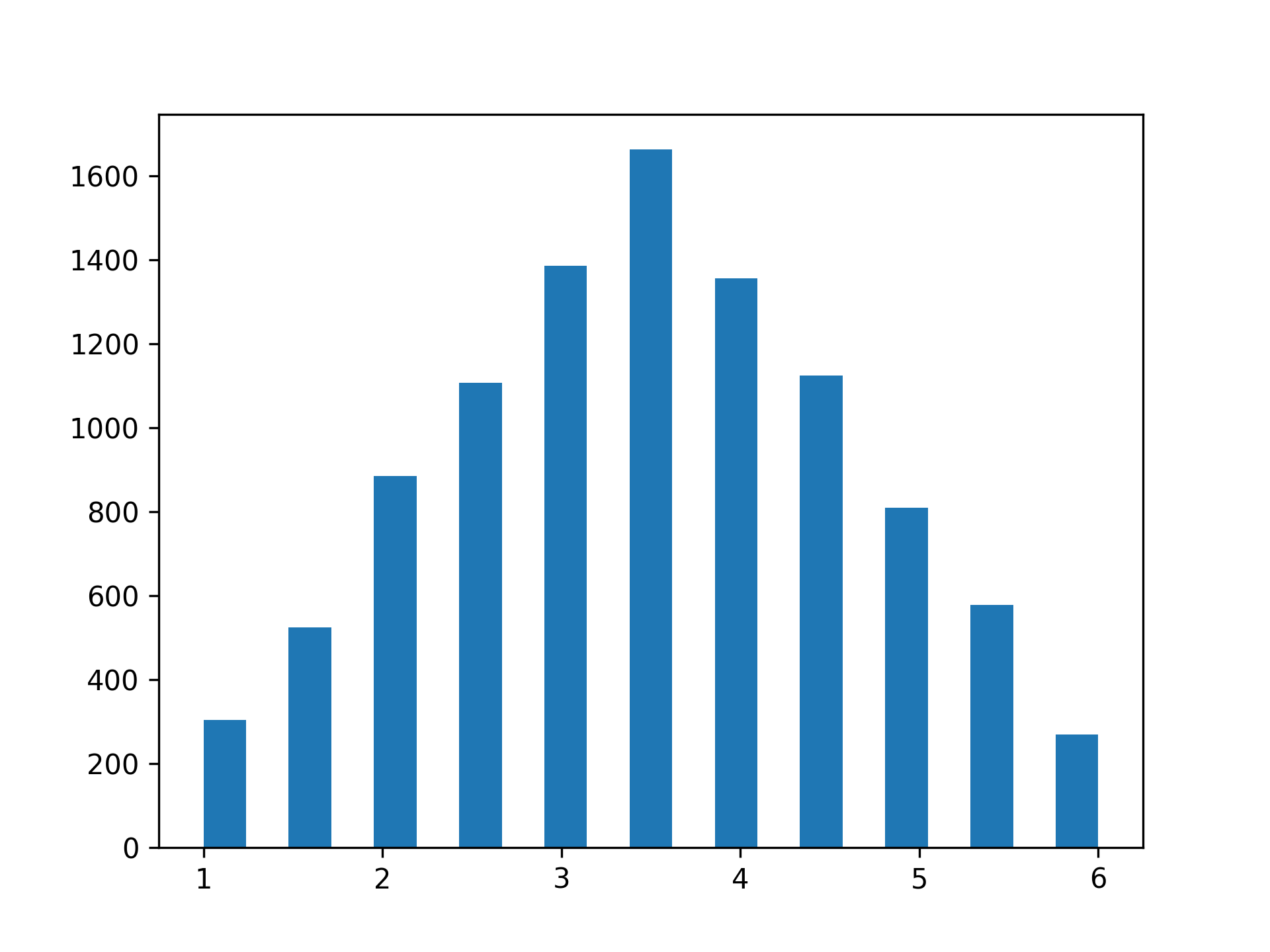
While the distribution is close to symmetrical and has a clear peak, you notice that the shape is more triangular than bell-shaped. At the same time, the distribution no longer shows uniformity, where each outcome would be equally likely.
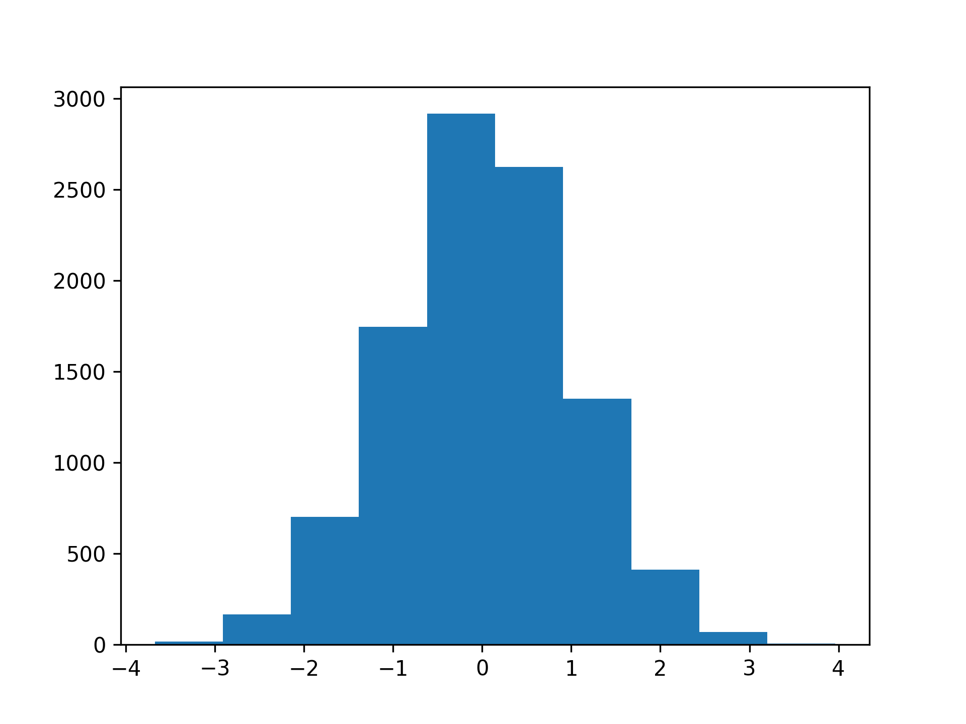
Next, try the same with ten repeated die rolls:
>>> rolls = rng.integers(low=1, high=6, endpoint=True, size=(10_000, 10))
>>> plt.hist(rolls.mean(axis=1), bins=41)
>>> plt.show()
Now, the distribution is much closer to the familiar shape:
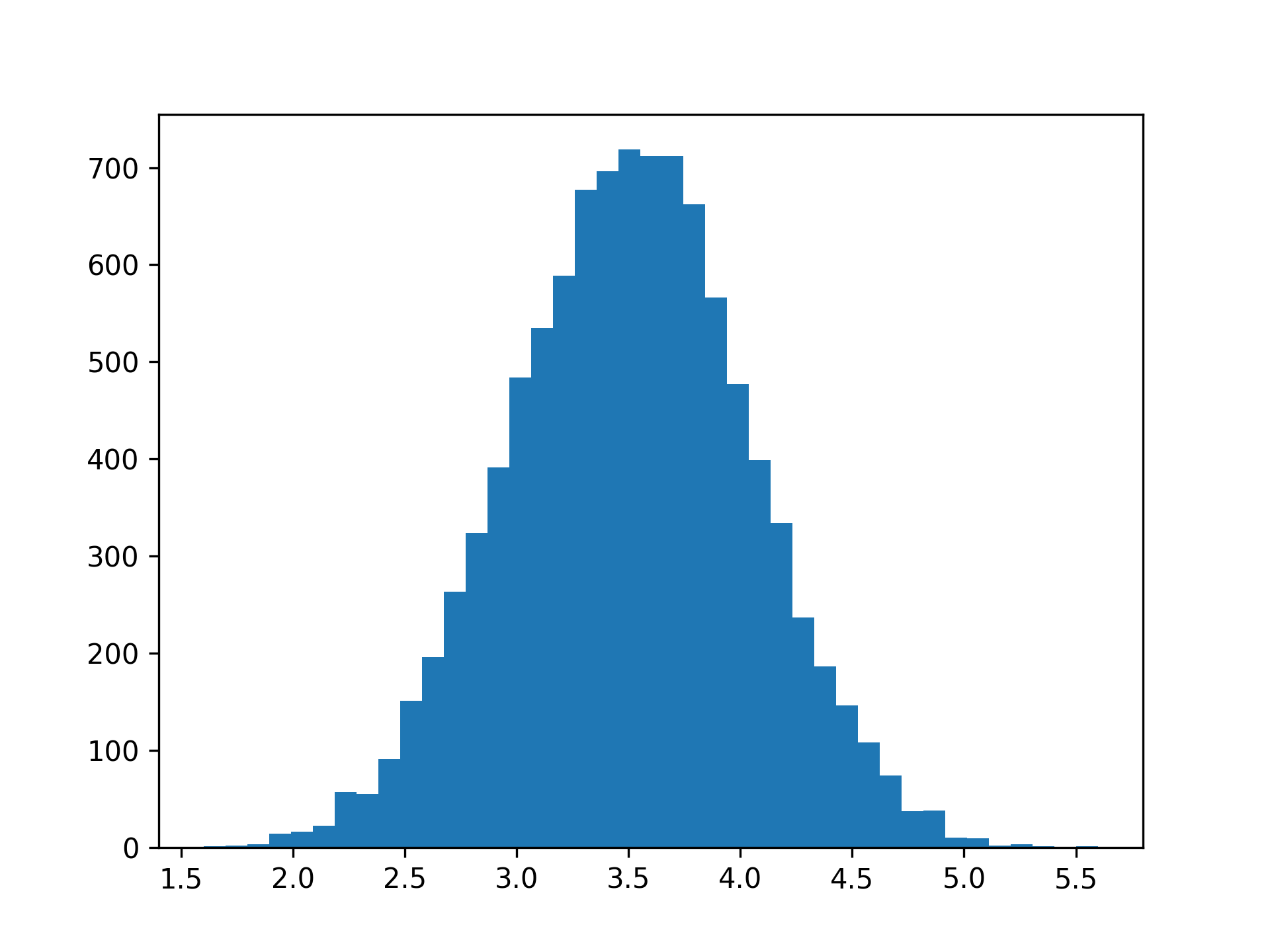
If you increase the number of repeated rolls, then you’ll see that the distribution will get ever closer to the normal distribution. This illustrates the central limit theorem: repeated experiments produce normality. Because many natural processes include additive effects, they often follow the normal distribution fairly well.
Conclusion
In this tutorial, you’ve learned how you can work with normally distributed data in NumPy, and how you can plot them in Matplotlib. The normal distribution is one of the most common probability distributions, and you’ve seen how you can visually compare the distribution of your sample data to the theoretical normal distribution.
The central limit theorem explains one reason why you can find the normal distribution everywhere. The average of repeated experiments tends toward normality.
Do you have an interesting example of normally distributed numbers? Share it with the community in the comments below.
Free Bonus: Click here to download the free sample code that you’ll use to generate random numbers from a normal distribution in NumPy.