How to Work With Polars LazyFrames

How to Create a Polars LazyFrame

You can create LazyFrames in three main ways:

1. From a data file using any of the available scan functions, such as scan_parquet() or scan_csv().
2. By passing a dictionary, a sequence such as a list, a NumPy array, or even a pandas DataFrame to the LazyFrame() constructor.
3. By using the .lazy() method to convert an existing Polars DataFrame to a LazyFrame.

The most common way to create a LazyFrame is by using one of the various scan functions to analyze your data file. You saw this in action earlier when you used scan_parquet() to create a LazyFrame based on the content of your rides.parquet file. You can also read other file formats lazily using functions such as scan_csv() and scan_ndjson().

A second way to create a LazyFrame is to pass the data you want to use to the LazyFrame() constructor. This is used for very small LazyFrames. The code below shows you how to create one from a dictionary:

>>> import polars as pl

>>> programming_languages = {
...     "language_id": range(5),
...     "language": ["Pascal", "C", "C++", "Python", "Java"],
...     "creator": [
...         "Niklaus Wirth",
...         "Dennis Ritchie",
...         "Bjarne Stroustrup",
...         "Guido van Rossum",
...         "James Gosling",
...     ],
...     "year": [1970, 1973, 1985, 1991, 1995],
... }

>>> pl.LazyFrame(programming_languages).collect()
shape: (5, 4)
┌─────────────┬──────────┬───────────────────┬──────┐
│ language_id ┆ language ┆ creator           ┆ year │
│ ---         ┆ ---      ┆ ---               ┆ ---  │
│ i64         ┆ str      ┆ str               ┆ i64  │
╞═════════════╪══════════╪═══════════════════╪══════╡
│ 0           ┆ Pascal   ┆ Niklaus Wirth     ┆ 1970 │
│ 1           ┆ C        ┆ Dennis Ritchie    ┆ 1973 │
│ 2           ┆ C++      ┆ Bjarne Stroustrup ┆ 1985 │
│ 3           ┆ Python   ┆ Guido van Rossum  ┆ 1991 │
│ 4           ┆ Java     ┆ James Gosling     ┆ 1995 │
└─────────────┴──────────┴───────────────────┴──────┘

You define a programming_languages dictionary that contains the data you want. The keys of your dictionary are used to form the column headings of the LazyFrame, while the dictionary values, which in this case are a range() object and three lists, form its data. This information is then used by Polars to construct the LazyFrame. To see data produced by the LazyFrame, you materialize it by calling .collect(), which produces the output shown.

When reading a data file, Polars applies a suitable data type to each of its columns, but this might not always be the most efficient choice. As you can see from the resulting DataFrame, the language_id and year columns have been read as 64-bit integers (i64), which are larger than needed. This wastes space.

In addition, Polars uses data type coercion. This means it’ll adjust the size of data internally to the minimum size needed to ensure an operation succeeds. For example, 64-bit integers may be coerced into 32-bit integers provided, of course, the calculation still works. This allows internal data processing to run on minimal required memory, but the output might still not be what you want.

Fortunately, it’s possible to define the data types you wish Polars to use. To do this, you can pass them in as a dictionary to the schema parameter of the LazyFrame() constructor:

>>> import polars as pl

>>> programming_languages = {
...     "language_id": range(5),
...     "language": ["Pascal", "C", "C++", "Python", "Java"],
...     "creator": [
...         "Niklaus Wirth",
...         "Dennis Ritchie",
...         "Bjarne Stroustrup",
...         "Guido van Rossum",
...         "James Gosling",
...     ],
...     "year": [1970, 1973, 1985, 1991, 1995],
... }

>>> d_types = {
...     "language_id": pl.Int32,
...     "language": pl.String,
...     "creator": pl.String,
...     "year": pl.Int32,
... }

>>> pl.LazyFrame(programming_languages, schema=d_types).collect()
shape: (5, 4)
┌─────────────┬──────────┬───────────────────┬──────┐
│ language_id ┆ language ┆ creator           ┆ year │
│ ---         ┆ ---      ┆ ---               ┆ ---  │
│ i32         ┆ str      ┆ str               ┆ i32  │
╞═════════════╪══════════╪═══════════════════╪══════╡
│ 0           ┆ Pascal   ┆ Niklaus Wirth     ┆ 1970 │
│ 1           ┆ C        ┆ Dennis Ritchie    ┆ 1973 │
│ 2           ┆ C++      ┆ Bjarne Stroustrup ┆ 1985 │
│ 3           ┆ Python   ┆ Guido van Rossum  ┆ 1991 │
│ 4           ┆ Java     ┆ James Gosling     ┆ 1995 │
└─────────────┴──────────┴───────────────────┴──────┘

This time, you create a d_types dictionary containing the data types you want. Its keys match the column headings defined in the programming_languages dictionary and the LazyFrame headings, while its values define the data types you desire. You then assign this second dictionary to the schema parameter of LazyFrame(). As with all LazyFrames, you must remember to materialize it to see its data, which you do with .collect().

As the highlighted line proves, both numeric columns are now 32-bit integers.

>>> pl.LazyFrame(programming_languages, schema=d_types).collect_schema()
Schema({'language_id': Int32, 'language': String,
⮑ 'creator': String, 'year': Int32})

If you want to write the analyzed results out to a file, then you can use one of several DataFrame methods such as .write_parquet() to do so. In the previous example, using lf.collect().write_parquet("analysis_results.parquet") would write your results into a parquet file. However, this only works if your DataFrame fits into your computer’s RAM and can be problematic otherwise. You’ll see how to avoid this later.

The third way to create a LazyFrame is to use the .lazy() method on a Polars DataFrame. You commonly use this to flip between eager mode, which uses DataFrames, and lazy mode. Some operations can’t work lazily because they need data to work with. However, you may want to apply further processing to a DataFrame that can make use of the LazyFrame efficiencies.

You’ll learn more about flipping between lazy and eager modes later, but for now, here’s how to use the .lazy() method on a DataFrame:

 1>>> languages_df = pl.read_csv("programming_languages.csv")
 2>>> type(languages_df)
 3<class 'polars.dataframe.frame.DataFrame'>
 4
 5>>> languages_lf = languages_df.lazy()
 6>>> type(languages_lf)
 7<class 'polars.lazyframe.frame.LazyFrame'>

This time, you use the read_csv() function to read the data contained within programming_languages.csv into languages_df. To confirm that you’ve created a DataFrame, you use the built-in type() function. As you can see from line 3, everything is as expected.

In line 5, you use .lazy() to transform languages_df into the languages_lf LazyFrame. As before, type() confirms that a LazyFrame is now present.

Now that you know how to create a LazyFrame, next you’ll delve a little deeper and see why they’re such cool tools.

How to Monitor LazyFrame Efficiency

While traditional DataFrames contain data, LazyFrames contain a set of instructions, known as a query plan, that define the operations that should be carried out on the data. As you saw earlier, you need to materialize the LazyFrame into a DataFrame to see the data. So why bother with LazyFrames? Why not just stick to the tried and trusted DataFrames? Here’s why!

The query plan of a LazyFrame is optimized for efficient analysis of the data source before any data is analyzed. The LazyFrame reads and processes the data only when it’s materialized. So, although your LazyFrame contains multiple instructions, no data is read until materialization, eliminating data read delays during its construction.

LazyFrames are the recommended way of working whenever possible. Unfortunately, there are exceptions where lazy mode isn’t an option and you’ll look at these later on. For now, you can put these to one side and concentrate on the positives.

To compare the efficiency of LazyFrames versus DataFrames, you’ll time an identical analysis of some data using both a LazyFrame and a DataFrame. To make sure that both examples end at the same position, you’ll call .collect() on the LazyFrame to make sure it reads the data after optimization.

In this first test, you’ll work with a DataFrame created by running read_parquet() on the rides.parquet file. Create the following Python file and name it dataframe_timer.py:

 1import time
 2import polars as pl
 3
 4start = time.perf_counter()
 5
 6for _ in range(10):
 7    rides = pl.read_parquet("rides.parquet")
 8    (
 9        rides
10        .filter(pl.col("pick_up") == pl.col("drop_off"))
11        .group_by(pl.col("pick_up"))
12        .agg(pl.col("fare").mean())
13        .filter(
14            pl.col("pick_up").is_in(
15                ["Brooklyn", "Bronx", "Queens", "Manhattan"]
16            )
17        )
18    )
19
20end = time.perf_counter()
21
22print(f"Code finished in {(end - start)/10:.4f} seconds.")

To time your Python code efficiently, you use perf_counter() from the built-in time module. This is a simple but accurate way of timing Python code. When you call time.perf_counter(), the function takes a reading from your computer’s clock. By doing this at the start and end of the test, you can work out how long the code is taking to run, and by averaging over ten iterations, you can improve the accuracy of the result.

When you run your code, you’ll see how long it took:

$ python dataframe_timer.py
Code finished in 0.1178 seconds.

When your code runs, it reads all of the data from the file into memory ten separate times, and each time repeats the same processing. As each processing step completes, the data in the result DataFrame changes until it mutates into its final form. Polars carries each step out on the DataFrame in the order they’re specified in the code. This might not be the best order of execution.

A combination of having to read all of the data into memory, the constant updates, and their inefficient order wastes the computer’s resources. As a consequence of this, the time taken to run this test is relatively slow, as you’ll see in the next test.

Next, you’ll repeat the previous test only this time, you’ll work with a LazyFrame. Create lazyframe_timer.py as follows:

import time
import polars as pl

start = time.perf_counter()

for _ in range(10):
    rides = pl.scan_parquet("rides.parquet")
    (
        rides
        .filter(pl.col("pick_up") == pl.col("drop_off"))
        .group_by(pl.col("pick_up"))
        .agg(pl.col("fare").mean())
        .filter(
            pl.col("pick_up").is_in(
                ["Brooklyn", "Bronx", "Queens", "Manhattan"]
            )
        )
    ).collect()

end = time.perf_counter()

print(f"Code finished in {(end - start)/10:.4f} seconds.")

To create the LazyFrame, you pass rides.parquet to scan_parquet() as highlighted, instead of to read_parquet() as before. To make sure both versions of your code produce a DataFrame, you also call the .collect() method to materialize it. Apart from these two changes, the rest of the code is identical.

Again, you run your code to time your LazyFrame:

$ python lazyframe_timer.py
Code finished in 0.0919 seconds.

This time, when you run your code, each processing step doesn’t process the data directly. Instead, it simply adds instructions. Remember, LazyFrames are nothing more than a set of instructions defining what’s to be done to the data.

When you call .collect() to see the result, the query won’t necessarily be applied to the data in the same order written in your code. Instead, Polars will optimize the LazyFrame before running it so that when the instructions are applied, they process the data efficiently. This ability of Polars to optimize its queries produces the faster time than that obtained earlier in your DataFrame test. You’ll learn more about how this is done next.

How LazyFrames Achieve Efficiency

In this section, you’ll take a look at how query plans are optimized before they’re run. This is the secret to LazyFrame efficiency. There are two types of query plans: the optimized query plan and the sub-optimized query plan. The optimized query plan is used by LazyFrames to process data as efficiently as possible, while the sub-optimized query plan is used by DataFrames to apply the query steps in the order they are defined in the code.

Investigating the Sub-Optimized Query Plan

Before you can understand how query plans are optimized, you need to learn how to view and read one. You’ll start with the sub-optimized version:

To see a query plan, you use LazyFrame.explain() to display it:

Python

 1>>> import polars as pl
 2
 3>>> rides = pl.scan_parquet("rides.parquet")
 4
 5>>> print(
 6...     (
 7...         rides
 8...         .filter(pl.col("pick_up") == pl.col("drop_off"))
 9...         .group_by(pl.col("pick_up"))
10...         .agg(pl.col("fare").mean())
11...         .filter(
12...             pl.col("pick_up").is_in(
13...                 ["Brooklyn", "Bronx", "Queens", "Manhattan"]
14...             )
15...         )
16...     ).explain(optimized=False)
17... )
18FILTER col("pick_up").is_in([Series]) FROM
19  AGGREGATE
20        [col("fare").mean()] BY [col("pick_up")] FROM
21    FILTER [(col("pick_up")) == (col("drop_off"))] FROM
22      Parquet SCAN [rides.parquet]
23      PROJECT */5 COLUMNS

In line 16, you requested that the sub-optimized plan be displayed by passing optimized=False to .explain(). Also, for clarity, you used the built in print() function in line 5. Without this, the output is less readable.

As you can see, the textual representation uses indentation to display the main query operations. The query plan consists of four main operations: FILTER, AGGREGATE, FILTER, and SCAN. While this can certainly be read, it can be a bit overwhelming the first time you see it. A better way is to use the free Graphviz software to render your query plans. This makes each step in the plan easier to visualize.

Installing GraphvizShow/Hide

If you want to display your query plans graphically, you must first install Graphviz. The specific procedure you follow will depend on your operating system:

• Windows
• Linux
• macOS

1. Download the latest Windows installer from the Graphviz download page. You’ll see the program is offered as both 32-bit and 64-bit executables. If you’re using Windows 11 or later, the 64-bit version is what you need. If you’re using an earlier edition of Windows and don’t know which to choose, try the 64-bit version first, and if that doesn’t work, the 32-bit version will.
2. Double-click the Windows installer file you downloaded to start the installation.
3. Click through the installation wizard, accepting the license agreement as you go. When you see the Install Options page, make sure Add Graphviz to the system PATH for the current user is selected.
4. Click Next until you reach the end of the installation wizard and Graphviz will be installed.
5. Although you won’t be prompted to do so, you should restart your computer to make sure the new environment variable has been read correctly.

The command you’ll use to install Graphviz will depend on the Linux distribution you’re using.

If you’re using either Debian or Ubuntu, run the following command:

Shell

$ sudo apt install graphviz

If you’re using either Fedora, RedHat, or CentOS, run the following command:

Shell

$ sudo dnf install graphviz

The graphviz program will now be available to you.

If you’re using macOS, run either of the following commands:

Shell

$ sudo port install graphviz

Or:

Shell

$ brew install graphviz

The graphviz program will now be available to you.

Once you’ve installed Graphviz, you’ll also need to install Matplotlib if you didn’t earlier. You can install the package using python -m pip install matplotlib. When both are installed, you can then use Graphviz to view query plans graphically.

Now you’ll take a look at the same query plan, only this time a graphical version:

Python

>>> import polars as pl

>>> rides = pl.scan_parquet("rides.parquet")

>>> (
...     rides
...     .filter(pl.col("pick_up") == pl.col("drop_off"))
...     .group_by(pl.col("pick_up"))
...     .agg(pl.col("fare").mean())
...     .filter(pl.col("pick_up")
...         .is_in(
...             ["Brooklyn", "Bronx", "Queens", "Manhattan"]
...         )
...     )
... ).show_graph(optimized=False)

Although your code creates the same LazyFrame as before, this time you replace .explain(optimized=False) with .show_graph(optimized=False) to display the sub-optimized query plan using Graphviz. This graphical version is shown below:

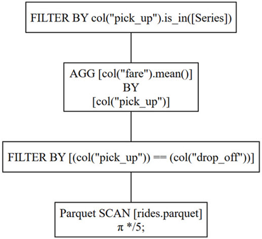
When you’re interpreting any query plan, it’s best to read it from the bottom up.

The bottom instruction means your code will first read all five columns from the rides.parquet file. The Greek letter pi (π) indicates a projection, which means that columns are to be read, while */5 specifies that your code will read all five columns.

Once the projection is complete, the next instruction up defines the first of the filter criteria your code will apply to the data. In this case, only those rows whose pick_up locations match their drop_off locations are considered.

When the correct rows have been determined, the grouping and aggregation comes next. As you learned earlier, your data is grouped by pick_up location before the mean fare is calculated.

Finally, you apply a second filter to include only those rows where the pick_up location values are within a series. Although the series is not specified in the plan, it refers to the four boroughs defined in the code.

It’s important to remember that since this query plan is the sub-optimal version, it’ll never be used by the LazyFrame. In this plan, the order of the steps mirror those of the code. This query plan is how the data would have been processed had you used .read_parquet() to create a DataFrame, instead of .scan_parquet() to create a LazyFrame.

Now that you’ve seen a graphical representation of a query plan, look back at the textual representation shown first and it’ll be easier to understand. As you can see, the textual representation uses indentation instead of boxes. However, each of the four indentations in the textual representation corresponds to one of the four individual boxes in the Graphviz diagram.

Now that you’ve been introduced to the idea of a query plan, next you’ll see how they’re actually used by LazyFrames.

Remove ads

Investigating the Optimized Query Plan

To understand what actually happens when you run LazyFrame code, you need to view the all-important, optimized query plan:

Python

>>> rides = pl.scan_parquet("rides.parquet")

>>> (
...     rides
...     .filter(pl.col("pick_up") == pl.col("drop_off"))
...     .group_by(pl.col("pick_up"))
...     .agg(pl.col("fare").mean())
...     .filter(pl.col("pick_up")
...         .is_in(
...             ["Brooklyn", "Bronx", "Queens", "Manhattan"]
...         )
...     )
... ).show_graph(optimized=True)

To view the optimized query plan, you pass optimized=True to either .show_graph(), or to .explain(). Despite this being only a small change, the effects are significant:

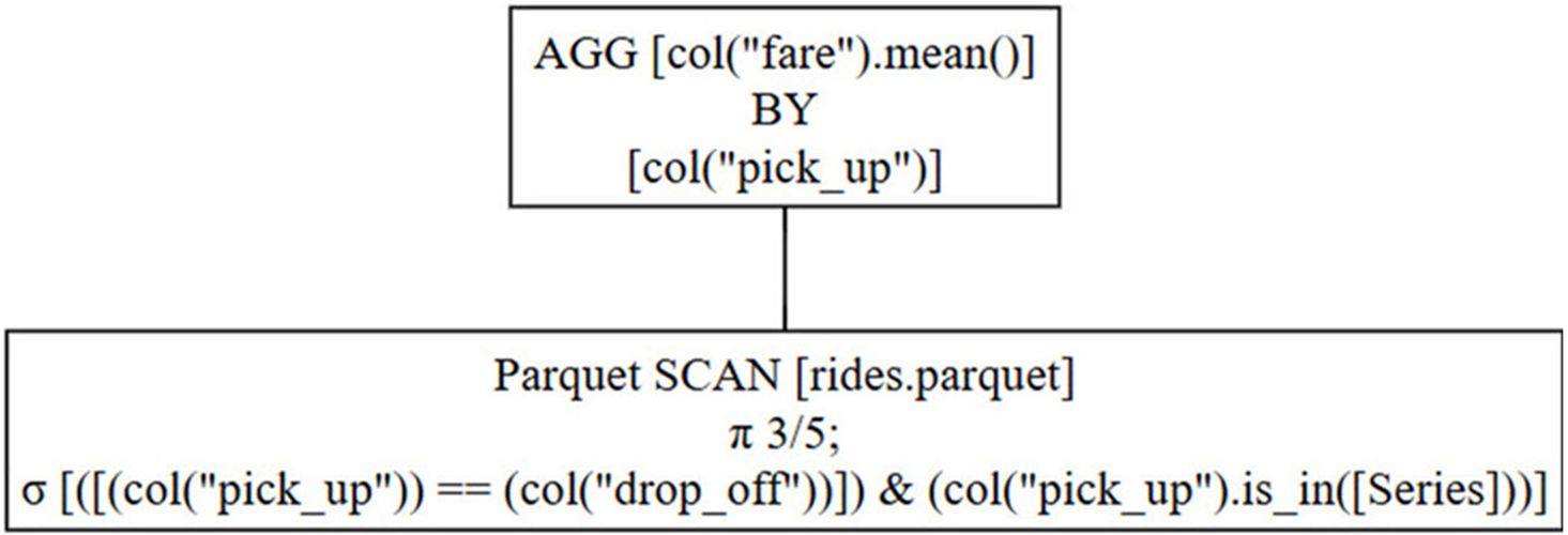
This time, Polars has merged both the original filters into a single selection instruction as annotated by the Greek letter sigma (σ). This means that right from the start of this optimized query, only those rows which are needed are actually read. When DataFrames are used, all rows are read. Moving the row selection to the start of the query is called predicate pushdown.

Notice that the projection instruction (π 3/5) means that Polars will read only three of the five columns, since these are all it needs. These are the pick_up, drop_off, and fare columns. Selecting only those columns necessary is called projection pushdown.

Once Polars has retrieved the data it needs, which will be quicker than reading all of it, it performs the same aggregation as before. However, with less data to process, the calculation runs faster, reducing the overall computational load.

In addition to both predicate and projection pushdown, the LazyFrame’s schema also plays a part in achieving efficiency. Polars consults the LazyFrame’s schema and uses it to verify the correctness of its optimized query plan before the query runs. In contrast, DataFrames read the data first and will only fail when they attempt to process it.

You can view the schema using .collect_schema():

Python

>>> rides.collect_schema()
Schema(
⮑ {'pick_up': String,
⮑ 'pu_time': Datetime(time_unit='ns', time_zone=None),
⮑ 'drop_off': String,
⮑ 'do_time': Datetime(time_unit='ns', time_zone=None),
⮑ 'passengers': Int32,
⮑ 'distance': Int32, 'fare': Int32}
⮑)

For example, there’d be no point in Polars working out the mean pick_up field value since it has a data type of String. The query will fail quickly because the optimized query knows this up front from the schema. Conversely, when DataFrames are used, .mean() will still fail, but only after reading the entire dataset, potentially wasting time and resources.

LazyFrames also achieve efficiency by running their query plans in parallel. This allows multiple operations in a plan to be run simultaneously, their results cached, and then combined together to produce a further result.

For example, if a query requires data from multiple files, it’s likely that each of the files will be read in parallel, and then both datasets analyzed together. Of course the LazyFrame efficiencies will be applied before each file read begins.

While these are the main ways Polars can optimize data analysis when working in lazy mode, it has several other tricks up its sleeve. Altogether, this means that working with LazyFrames should be your first choice whenever possible.

So far, the code examples assume that all your data can fit within your computer’s memory for processing. Next, you’ll see how Polars can be made to cope when it doesn’t.

How LazyFrames Cope With Large Volumes of Data

LazyFrames use something called streaming to allow them to work with large volumes of data. Streaming allows LazyFrames to deal with data that would otherwise be too large to fit into RAM. In this section, you’ll learn how it works, when to use it, and when not to.

$ python taxi_rides_80GB.py

$ dir 2021_Yellow_Taxi_Trip_Data.csv

$ ls -l 2021_Yellow_Taxi_Trip_Data.csv

>>> import polars as pl

>>> rides = pl.scan_csv("2021_Yellow_Taxi_Trip_Data.csv")

>>> print(
...     (
...         rides
...         .group_by(pl.col("PULocationID"))
...         .agg(pl.col("total_amount").sum())
...     ).collect(streaming=True)
... )
shape: (265, 2)
┌──────────────┬──────────────┐
│ PULocationID ┆ total_amount │
│ ---          ┆ ---          │
│ i64          ┆ f64          │
╞══════════════╪══════════════╡
│ 197          ┆ 2.2632e8     │
│ 176          ┆ 2.2658e8     │
│ 212          ┆ 2.2638e8     │
│ 236          ┆ 2.2647e8     │
│ 209          ┆ 2.2639e8     │
│ …            ┆ …            │
│ 207          ┆ 2.2643e8     │
│ 187          ┆ 2.2648e8     │
│ 43           ┆ 2.2647e8     │
│ 82           ┆ 2.2633e8     │
│ 175          ┆ 2.2617e8     │
└──────────────┴──────────────┘

 1>>> import polars as pl
 2
 3>>> rides = pl.scan_parquet("rides.parquet")
 4
 5>>> print(
 6...     (
 7...         rides
 8...         .filter(pl.col("pick_up") == pl.col("drop_off"))
 9...         .group_by(pl.col("pick_up"))
10...         .agg(pl.col("drop_off").mean())
11...         .filter(
12...             pl.col("pick_up").is_in(
13...                 ["Brooklyn", "Bronx", "Queens", "Manhattan"]
14...             )
15...         )
16...     ).explain(streaming=True, optimized=True)
17... )
18STREAMING:
19  AGGREGATE
20        [col("drop_off").mean()] BY [col("pick_up")] FROM
21    Parquet SCAN [rides.parquet]
22    PROJECT 2/5 COLUMNS
23    SELECTION: [([(col("pick_up")) == (col("drop_off"))])
24⮑  & (col("pick_up").is_in([Series]))]

>>> import polars as pl

>>> rides = pl.scan_parquet("rides.parquet")

>>> print(
...     (
...         rides
...         .filter(pl.col("pick_up") == pl.col("drop_off"))
...         .with_columns(
...             pl.col("fare")
...             .mean()
...             .over(pl.col("pick_up"))
...             .alias("mean fare")
...         )
...     ).explain(streaming=True, optimized=True)
... )
 WITH_COLUMNS:
 [col("fare").mean().over([col("pick_up")]).alias("mean fare")]
  STREAMING:
    Parquet SCAN [rides.parquet]
    PROJECT */5 COLUMNS
    SELECTION: [(col("pick_up")) == (col("drop_off"))]

How to Decide if LazyFrames Are Suitable

At this point, you’ve learned about the many benefits that LazyFrames provide over DataFrames. Indeed, you may even be wondering why anyone would want to work with DataFrames at all. However, while LazyFrames are powerful, they’re not always suitable because some processing requires the underlying data to be present in a DataFrame before it’ll work.

A pivot table is a common tool used in data analysis to summarize large volumes of data by grouping it into categories and performing an aggregation on those categories. Suppose you wanted to see the total passengers carried between the different locations. You could do this using a pivot table:

>>> import polars as pl

>>> rides = pl.scan_parquet("rides.parquet")

>>> (
...     rides
...     .pivot(
...         on="pick_up",
...         index="drop_off",
...         values="passengers",
...         aggregate_function="sum",
...     )
... )
Traceback (most recent call last):
  ...
AttributeError: 'LazyFrame' object has no attribute 'pivot'.
⮑ Did you mean: 'unpivot'?

In this code, you’ve attempted to create a LazyFrame that will contain a separate column for each pick_up, and a separate row for each drop_off. At each row/column intersection, the sum of the number of passengers transported between them should be calculated. Unfortunately, the code failed with an AttributeError because LazyFrames don’t support .pivot().

To fix this, you need to use a DataFrame:

>>> (
...     rides
...     .collect()
...     .pivot(
...         on="pick_up",
...         index="drop_off",
...         values="passengers",
...         aggregate_function="sum",
...     )
... )
shape: (8, 9)
┌───────────────┬───────────┬────────┬─────────┬───┬
│ drop_off      ┆ Manhattan ┆ Queens ┆ Unknown ┆ … ┆
│ ---           ┆ ---       ┆ ---    ┆ ---     ┆   ┆
│ str           ┆ i32       ┆ i32    ┆ i32     ┆   ┆
╞═══════════════╪═══════════╪════════╪═════════╪═══╪
│ Manhattan     ┆ 3041648   ┆ 256376 ┆ 4686    ┆ … ┆
│ Queens        ┆ 111178    ┆ 115640 ┆ 629     ┆ … ┆
│ Brooklyn      ┆ 68712     ┆ 66116  ┆ 333     ┆ … ┆
│ Bronx         ┆ 12006     ┆ 10396  ┆ 59      ┆ … ┆
│ Unknown       ┆ 9668      ┆ 1016   ┆ 7512    ┆ … ┆
│ N/A           ┆ 6312      ┆ 17630  ┆ 66      ┆ … ┆
│ Staten Island ┆ 346       ┆ 718    ┆ 2       ┆ … ┆
│ EWR           ┆ 12759     ┆ 806    ┆ 27      ┆ … ┆
└───────────────┴───────────┴────────┴─────────┴───┴
┬──────┬───────┬──────┬───────────────┐
┆ N/A  ┆ Bronx ┆ EWR  ┆ Staten Island │
┆ ---  ┆ ---   ┆ ---  ┆ ---           │
┆ i32  ┆ i32   ┆ i32  ┆ i32           │
╪══════╪═══════╪══════╪═══════════════╡
┆ 113  ┆ 3749  ┆ 14   ┆ 11            │
┆ 148  ┆ 830   ┆ 1    ┆ 3             │
┆ 20   ┆ 924   ┆ 1    ┆ 38            │
┆ 23   ┆ 1785  ┆ null ┆ null          │
┆ 37   ┆ 13    ┆ 10   ┆ null          │
┆ 2974 ┆ 82    ┆ 25   ┆ 5             │
┆ null ┆ null  ┆ null ┆ 45            │
┆ 131  ┆ 6     ┆ 1034 ┆ 3             │
┴──────┴───────┴──────┴───────────────┘

This time, everything works as expected. Even though you started out with a LazyFrame, because you called .collect() on it to materialize it, the .pivot() method worked as expected because it was using actual data stored in a DataFrame. DataFrames are quite happy using .pivot(), so the code ran without error. You have the result you want, which has been split into two parts for display purposes.

To maximize efficiency, you can also run part of an analysis query in lazy mode and part in eager mode. Although you’re happy with the result above, suppose you decide you only want to see the details for Brooklyn, Bronx, and Queens. To do this, you again use filter():

 1>>> boroughs = ["Brooklyn", "Bronx", "Queens"]
 2>>> (
 3...     rides
 4...     .filter(pl.col("pick_up").is_in(boroughs))
 5...     .filter(pl.col("drop_off").is_in(boroughs))
 6...     .collect()
 7...     .pivot(
 8...         on="pick_up",
 9...         index="drop_off",
10...         values="passengers",
11...         aggregate_function="sum",
12...     )
13... )
14shape: (3, 4)
15┌─────────────┬────────┬──────────┬───────┐
16│ drop_off    ┆ Queens ┆ Brooklyn ┆ Bronx │
17│ ---         ┆ ---    ┆ ---      ┆ ---   │
18│ str         ┆ i32    ┆ i32      ┆ i32   │
19╞═════════════╪════════╪══════════╪═══════╡
20│ Brooklyn    ┆ 66116  ┆ 18854    ┆ 924   │
21│ Queens      ┆ 115640 ┆ 3442     ┆ 830   │
22│ Bronx       ┆ 10396  ┆ 862      ┆ 1785  │
23└─────────────┴────────┴──────────┴───────┘

As you saw earlier, .filter() can operate on LazyFrames so you can apply it here. In the example above, this means that lines 3 through 5 will run optimally in lazy mode. Then, because .pivot() can’t work in lazy mode, you call .collect() to create a DataFrame containing the data for pivot() to work with. This time, .pivot() will only be using the data from the three desired locations.

Had there been further processing that did support lazy mode, but that first required a DataFrame to be present, you’d flip things back across using .lazy().

For example, suppose you want to add additional analysis that allows you to view only the row where the maximum number of passengers appears. You can do this using .select(). While .select() works in both eager and lazy mode, you should work lazily whenever possible:

>>> boroughs = ["Brooklyn", "Bronx", "Queens"]
>>> (
...     rides
...     .filter(pl.col("pick_up").is_in(boroughs))
...     .filter(pl.col("drop_off").is_in(boroughs))
...     .collect()
...     .pivot(
...         on="pick_up",
...         index="drop_off",
...         values="passengers",
...         aggregate_function="sum",
...     )
...     .lazy()
...     .select(pl.max("*"))
... ).collect()
shape: (1, 4)
┌─────────────┬────────┬──────────┬───────┐
│ drop_off    ┆ Queens ┆ Brooklyn ┆ Bronx │
│ ---         ┆ ---    ┆ ---      ┆ ---   │
│ str         ┆ i32    ┆ i32      ┆ i32   │
╞═════════════╪════════╪══════════╪═══════╡
│ Queens      ┆ 115640 ┆ 18854    ┆ 1785  │
└─────────────┴────────┴──────────┴───────┘

To allow .select() to work in the more desirable lazy mode, you flip the query back into lazy mode using .lazy() as highlighted. Once you’re working lazily again, you use .select(pl.max("*")) to select the row containing the highest value. In this case, it’s the row containing 115640. You also remembered to use .collect() to materialize the data—otherwise, you’d only see the LazyFrame object with its sub-optimized query plan.

>>> df_ops = {
...     x for x in dir(pl.DataFrame()) if not x.startswith("_")
... }
>>> lazy_ops = {
...     x for x in dir(pl.LazyFrame()) if not x.startswith("_")
... }
>>> print(sorted(df_ops - lazy_ops))
['corr', 'drop_in_place', 'equals', 'estimated_size', 'extend', 'flags',
⮑ 'fold', 'get_column', 'get_column_index', 'get_columns', 'glimpse',
⮑ 'hash_rows`, 'height', 'hstack', 'insert_column', 'is_duplicated',
⮑ 'is_empty', 'is_unique', ... ]

Congratulations on completing this tutorial. You can now look forward to using LazyFrames to analyze your data efficiently.

Conclusion

In this tutorial, you’ve learned how to work with Polars LazyFrames. To begin with, you learned how to create one before diving a little deeper to understand how they achieve efficiency. You then learned the techniques that allow your LazyFrames to deal with large volumes of data before wrapping up with an understanding of their limitations.

As you can see, LazyFrames may not solve every data analysis problem, but they do provide an efficient solution for many. Looking forward, Polars is a library that’s still growing and its capabilities are expanding. Be sure to keep an eye on the latest developments in this exciting data analysis tool.

Take the Quiz: Test your knowledge with our interactive “How to Work With Polars LazyFrames” quiz. You’ll receive a score upon completion to help you track your learning progress:

---

Interactive Quiz

How to Work With Polars LazyFrames

This quiz will challenge your knowledge of working with Polars LazyFrames. You won't find all the answers in the tutorial, so you'll need to do some extra investigating. By finding all the answers, you're sure to learn some interesting things along the way.

Frequently Asked Questions

Now that you have some experience with Polars LazyFrames in Python, you can use the questions and answers below to check your understanding and recap what you’ve learned.

These FAQs are related to the most important concepts you’ve covered in this tutorial. Click the Show/Hide toggle beside each question to reveal the answer.