
The pandas DataFrame is a structure that contains two-dimensional data and its corresponding labels. DataFrames are widely used in data science, machine learning, scientific computing, and many other data-intensive fields.
DataFrames are similar to SQL tables or the spreadsheets that you work with in Excel or Calc. In many cases, DataFrames are faster, easier to use, and more powerful than tables or spreadsheets because they’re an integral part of the Python and NumPy ecosystems.
Take the Quiz: Test your knowledge with our interactive “The pandas DataFrame: Make Working With Data Delightful” quiz. You’ll receive a score upon completion to help you track your learning progress:

Interactive Quiz
The pandas DataFrame: Make Working With Data DelightfulTest your pandas skills! Practice DataFrame basics, column access, creation, sorting, and data manipulation in this interactive quiz.
In this tutorial, you’ll learn:
- What a pandas DataFrame is and how to create one
- How to access, modify, add, sort, filter, and delete data
- How to handle missing values
- How to work with time-series data
- How to quickly visualize data
It’s time to get started with pandas DataFrames!
Free Bonus: 5 Thoughts On Python Mastery, a free course for Python developers that shows you the roadmap and the mindset you’ll need to take your Python skills to the next level.
Introducing the pandas DataFrame
pandas DataFrames are data structures that contain:
- Data organized in two dimensions, rows and columns
- Labels that correspond to the rows and columns
You can start working with DataFrames by importing pandas:
>>> import pandas as pd
Now that you have pandas imported, you can work with DataFrames.
Imagine you’re using pandas to analyze data about job candidates for a position developing web applications with Python. Say you’re interested in the candidates’ names, cities, ages, and scores on a Python programming test, or py-score:
name |
city |
age |
py-score |
|
|---|---|---|---|---|
101 |
Xavier |
Mexico City |
41 |
88.0 |
102 |
Ann |
Toronto |
28 |
79.0 |
103 |
Jana |
Prague |
33 |
81.0 |
104 |
Yi |
Shanghai |
34 |
80.0 |
105 |
Robin |
Manchester |
38 |
68.0 |
106 |
Amal |
Cairo |
31 |
61.0 |
107 |
Nori |
Osaka |
37 |
84.0 |
In this table, the first row contains the column labels (name, city, age, and py-score). The first column holds the row labels (101, 102, and so on). All other cells are filled with the data values.
Now you have everything you need to create a pandas DataFrame.
There are several ways to create a pandas DataFrame. In most cases, you’ll use the DataFrame constructor and provide the data, labels, and other information. You can pass the data as a two-dimensional list, tuple, or NumPy array. You can also pass it as a dictionary or pandas Series instance, or as one of several other data types not covered in this tutorial.
For this example, assume you’re using a dictionary to pass the data:
>>> data = {
...     'name': ['Xavier', 'Ann', 'Jana', 'Yi', 'Robin', 'Amal', 'Nori'],
...     'city': ['Mexico City', 'Toronto', 'Prague', 'Shanghai',
...              'Manchester', 'Cairo', 'Osaka'],
...     'age': [41, 28, 33, 34, 38, 31, 37],
...     'py-score': [88.0, 79.0, 81.0, 80.0, 68.0, 61.0, 84.0]
... }

>>> row_labels = [101, 102, 103, 104, 105, 106, 107]
data is a Python variable that refers to the dictionary that holds your candidate data. It also contains the labels of the columns:
'name''city''age''py-score'
Finally, row_labels refers to a list that contains the labels of the rows, which are numbers ranging from 101 to 107.
Now you’re ready to create a pandas DataFrame:
>>> df = pd.DataFrame(data=data, index=row_labels)
>>> df
       name         city  age  py-score
101  Xavier  Mexico City   41      88.0
102     Ann      Toronto   28      79.0
103    Jana       Prague   33      81.0
104      Yi     Shanghai   34      80.0
105   Robin   Manchester   38      68.0
106    Amal        Cairo   31      61.0
107    Nori        Osaka   37      84.0
That’s it! df is a variable that holds the reference to your pandas DataFrame. This pandas DataFrame looks just like the candidate table above and has the following features:
- Row labels from
101to107 - Column labels such as
'name','city','age', and'py-score' - Data such as candidate names, cities, ages, and Python test scores
This figure shows the labels and data from df:
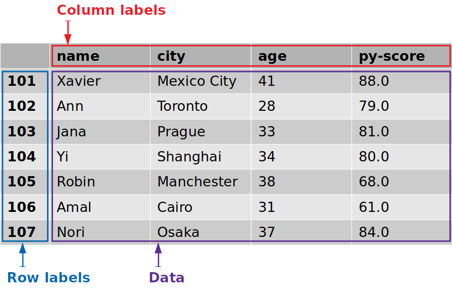
The row labels are outlined in blue, whereas the column labels are outlined in red, and the data values are outlined in purple.
pandas DataFrames can sometimes be very large, making it impractical to look at all the rows at once. You can use .head() to show the first few items and .tail() to show the last few items:
>>> df.head(n=2)
       name         city  age  py-score
101  Xavier  Mexico City   41      88.0
102     Ann      Toronto   28      79.0

>>> df.tail(n=2)
     name   city  age  py-score
106  Amal  Cairo   31      61.0
107  Nori  Osaka   37      84.0
That’s how you can show just the beginning or end of a pandas DataFrame. The parameter n specifies the number of rows to show.
Note: It may be helpful to think of the pandas DataFrame as a dictionary of columns, or pandas Series, with many additional features.
You can access a column in a pandas DataFrame the same way you would get a value from a dictionary:
>>> cities = df['city']
>>> cities
101    Mexico City
102        Toronto
103         Prague
104       Shanghai
105     Manchester
106          Cairo
107          Osaka
Name: city, dtype: object
This is the most convenient way to get a column from a pandas DataFrame.
If the name of the column is a string that is a valid Python identifier, then you can use dot notation to access it. That is, you can access the column the same way you would get the attribute of a class instance:
>>> df.city
101    Mexico City
102        Toronto
103         Prague
104       Shanghai
105     Manchester
106          Cairo
107          Osaka
Name: city, dtype: object
That’s how you get a particular column. You’ve extracted the column that corresponds with the label 'city', which contains the locations of all your job candidates.
It’s important to notice that you’ve extracted both the data and the corresponding row labels:
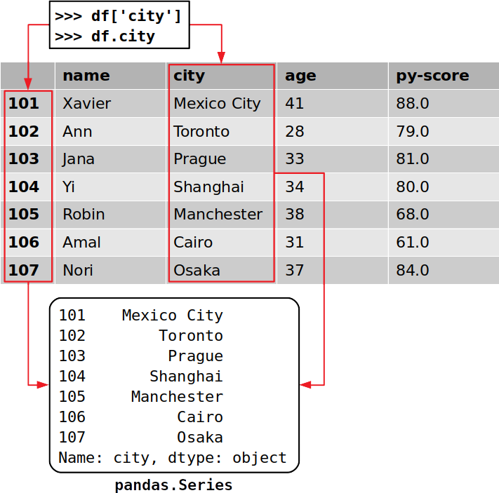
Each column of a pandas DataFrame is an instance of pandas.Series, a structure that holds one-dimensional data and their labels. You can get a single item of a Series object the same way you would with a dictionary, by using its label as a key:
>>> cities[102]
'Toronto'
In this case, 'Toronto' is the data value and 102 is the corresponding label. As you’ll see in a later section, there are other ways to get a particular item in a pandas DataFrame.
You can also access a whole row with the accessor .loc[]:
>>> df.loc[103]
name          Jana
city        Prague
age             33
py-score        81
Name: 103, dtype: object
This time, you’ve extracted the row that corresponds to the label 103, which contains the data for the candidate named Jana. In addition to the data values from this row, you’ve extracted the labels of the corresponding columns:
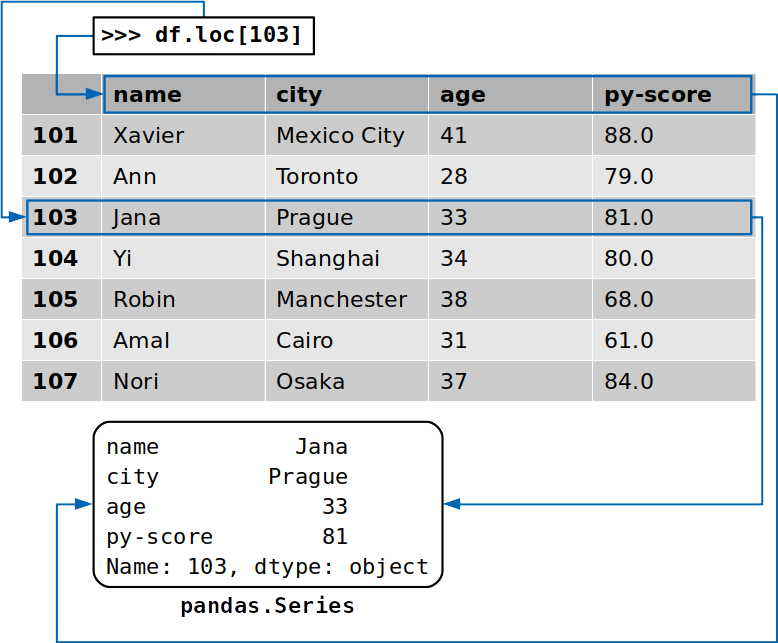
The returned row is also an instance of pandas.Series.
Creating a pandas DataFrame
As already mentioned, there are several way to create a pandas DataFrame. In this section, you’ll learn to do this using the DataFrame constructor along with:
- Python dictionaries
- Python lists
- Two-dimensional NumPy arrays
- Files
There are other methods as well, which you can learn about in the official documentation.
You can start by importing pandas along with NumPy, which you’ll use throughout the following examples:
>>> import numpy as np
>>> import pandas as pd
That’s it. Now you’re ready to create some DataFrames.
Creating a pandas DataFrame With Dictionaries
As you’ve already seen, you can create a pandas DataFrame with a Python dictionary:
>>> d = {'x': [1, 2, 3], 'y': np.array([2, 4, 8]), 'z': 100}

>>> pd.DataFrame(d)
   x  y    z
0  1  2  100
1  2  4  100
2  3  8  100
The keys of the dictionary are the DataFrame’s column labels, and the dictionary values are the data values in the corresponding DataFrame columns. The values can be contained in a tuple, list, one-dimensional NumPy array, pandas Series object, or one of several other data types. You can also provide a single value that will be copied along the entire column.
It’s possible to control the order of the columns with the columns parameter and the row labels with index:
>>> pd.DataFrame(d, index=[100, 200, 300], columns=['z', 'y', 'x'])
       z  y  x
100  100  2  1
200  100  4  2
300  100  8  3
As you can see, you’ve specified the row labels 100, 200, and 300. You’ve also forced the order of columns: z, y, x.
Creating a pandas DataFrame With Lists
Another way to create a pandas DataFrame is to use a list of dictionaries:
>>> l = [{'x': 1, 'y': 2, 'z': 100},
...      {'x': 2, 'y': 4, 'z': 100},
...      {'x': 3, 'y': 8, 'z': 100}]

>>> pd.DataFrame(l)
   x  y    z
0  1  2  100
1  2  4  100
2  3  8  100
Again, the dictionary keys are the column labels, and the dictionary values are the data values in the DataFrame.
You can also use a nested list, or a list of lists, as the data values. If you do, then it’s wise to explicitly specify the labels of columns, rows, or both when you create the DataFrame:
>>> l = [[1, 2, 100],
...      [2, 4, 100],
...      [3, 8, 100]]

>>> pd.DataFrame(l, columns=['x', 'y', 'z'])
   x  y    z
0  1  2  100
1  2  4  100
2  3  8  100
That’s how you can use a nested list to create a pandas DataFrame. You can also use a list of tuples in the same way. To do so, just replace the nested lists in the example above with tuples.
Creating a pandas DataFrame With NumPy Arrays
You can pass a two-dimensional NumPy array to the DataFrame constructor the same way you do with a list:
>>> arr = np.array([[1, 2, 100],
...                 [2, 4, 100],
...                 [3, 8, 100]])

>>> df_ = pd.DataFrame(arr, columns=['x', 'y', 'z'])
>>> df_
   x  y    z
0  1  2  100
1  2  4  100
2  3  8  100
Although this example looks almost the same as the nested list implementation above, it has one advantage: You can specify the optional parameter copy.
When copy is set to False (its default setting), the data from the NumPy array isn’t copied. This means that the original data from the array is assigned to the pandas DataFrame. If you modify the array, then your DataFrame will change too:
>>> arr[0, 0] = 1000

>>> df_
      x  y    z
0  1000  2  100
1     2  4  100
2     3  8  100
As you can see, when you change the first item of arr, you also modify df_.
Note: Not copying data values can save you a significant amount of time and processing power when working with large datasets.
If this behavior isn’t what you want, then you should specify copy=True in the DataFrame constructor. That way, df_ will be created with a copy of the values from arr instead of the actual values.
Creating a pandas DataFrame From Files
You can save and load the data and labels from a pandas DataFrame to and from a number of file types, including CSV, Excel, SQL, JSON, and more. This is a very powerful feature.
You can save your job candidate DataFrame to a CSV file with .to_csv():
>>> df.to_csv('data.csv')
The statement above will produce a CSV file called data.csv in your working directory:
,name,city,age,py-score
101,Xavier,Mexico City,41,88.0
102,Ann,Toronto,28,79.0
103,Jana,Prague,33,81.0
104,Yi,Shanghai,34,80.0
105,Robin,Manchester,38,68.0
106,Amal,Cairo,31,61.0
107,Nori,Osaka,37,84.0
Now that you have a CSV file with data, you can load it with read_csv():
>>> pd.read_csv('data.csv', index_col=0)
       name         city  age  py-score
101  Xavier  Mexico City   41      88.0
102     Ann      Toronto   28      79.0
103    Jana       Prague   33      81.0
104      Yi     Shanghai   34      80.0
105   Robin   Manchester   38      68.0
106    Amal        Cairo   31      61.0
107    Nori        Osaka   37      84.0
That’s how you get a pandas DataFrame from a file. In this case, index_col=0 specifies that the row labels are located in the first column of the CSV file.
Retrieving Labels and Data
Now that you’ve created your DataFrame, you can start retrieving information from it. With pandas, you can perform the following actions:
- Retrieve and modify row and column labels as sequences
- Represent data as NumPy arrays
- Check and adjust the data types
- Analyze the size of
DataFrameobjects
pandas DataFrame Labels as Sequences
You can get the DataFrame’s row labels with .index and its column labels with .columns:
>>> df.index
Int64Index([1, 2, 3, 4, 5, 6, 7], dtype='int64')

>>> df.columns
Index(['name', 'city', 'age', 'py-score'], dtype='object')
Now you have the row and column labels as special kinds of sequences. As you can with any other Python sequence, you can get a single item:
>>> df.columns[1]
'city'
In addition to extracting a particular item, you can apply other sequence operations, including iterating through the labels of rows or columns. However, this is rarely necessary since pandas offers other ways to iterate over DataFrames, which you’ll see in a later section.
You can also use this approach to modify the labels:
>>> df.index = np.arange(10, 17)

>>> df.index
Int64Index([10, 11, 12, 13, 14, 15, 16], dtype='int64')

>>> df
      name         city  age  py-score
10  Xavier  Mexico City   41      88.0
11     Ann      Toronto   28      79.0
12    Jana       Prague   33      81.0
13      Yi     Shanghai   34      80.0
14   Robin   Manchester   38      68.0
15    Amal        Cairo   31      61.0
16    Nori        Osaka   37      84.0
In this example, you use numpy.arange() to generate a new sequence of row labels that holds the integers from 10 to 16. To learn more about arange(), check out NumPy arange(): How to Use np.arange().
Keep in mind that if you try to modify a particular item of .index or .columns, then you’ll get a TypeError.
Data as NumPy Arrays
Sometimes you might want to extract data from a pandas DataFrame without its labels. To get a NumPy array with the unlabeled data, you can use either .to_numpy() or .values:
>>> df.to_numpy()
array([['Xavier', 'Mexico City', 41, 88.0],
       ['Ann', 'Toronto', 28, 79.0],
       ['Jana', 'Prague', 33, 81.0],
       ['Yi', 'Shanghai', 34, 80.0],
       ['Robin', 'Manchester', 38, 68.0],
       ['Amal', 'Cairo', 31, 61.0],
       ['Nori', 'Osaka', 37, 84.0]], dtype=object)
Both .to_numpy() and .values work similarly, and they both return a NumPy array with the data from the pandas DataFrame:
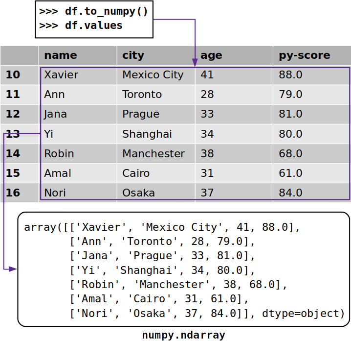
The pandas documentation suggests using .to_numpy() because of the flexibility offered by two optional parameters:
dtype: Use this parameter to specify the data type of the resulting array. It’s set toNoneby default.copy: Set this parameter toFalseif you want to use the original data from the DataFrame. Set it toTrueif you want to make a copy of the data.
However, .values has been around for much longer than .to_numpy(), which was introduced in pandas version 0.24.0. That means you’ll probably see .values more often, especially in older code.
Data Types
The types of the data values, also called data types or dtypes, are important because they determine the amount of memory your DataFrame uses, as well as its calculation speed and level of precision.
pandas relies heavily on NumPy data types. However, pandas 1.0 introduced some additional types:
BooleanDtypeandBooleanArraysupport missing Boolean values and Kleene three-value logic.StringDtypeandStringArrayrepresent a dedicated string type.
You can get the data types for each column of a pandas DataFrame with .dtypes:
>>> df.dtypes
name         object
city         object
age           int64
py-score    float64
dtype: object
As you can see, .dtypes returns a Series object with the column names as labels and the corresponding data types as values.
If you want to modify the data type of one or more columns, then you can use .astype():
>>> df_ = df.astype(dtype={'age': np.int32, 'py-score': np.float32})
>>> df_.dtypes
name         object
city         object
age           int32
py-score    float32
dtype: object
The most important and only mandatory parameter of .astype() is dtype. It expects a data type or dictionary. If you pass a dictionary, then the keys are the column names and the values are your desired corresponding data types.
As you can see, the data types for the columns age and py-score in the DataFrame df are both int64, which represents 64-bit (or 8-byte) integers. However, df_ also offers a smaller, 32-bit (4-byte) integer data type called int32.
pandas DataFrame Size
The attributes .ndim, .shape, and .size return the number of dimensions, number of data values across each dimension, and total number of data values, respectively:
>>> df_.ndim
2

>>> df_.shape
(7, 4)

>>> df_.size
28
DataFrame instances have two dimensions (rows and columns), so .ndim returns 2. A Series object, on the other hand, has only a single dimension, so in that case, .ndim would return 1.
The .shape attribute returns a tuple with the number of rows (in this case 7) and the number of columns (4). Finally, .size returns an integer equal to the number of values in the DataFrame (28).
You can even check the amount of memory used by each column with .memory_usage():
>>> df_.memory_usage()
Index       56
name        56
city        56
age         28
py-score    28
dtype: int64
As you can see, .memory_usage() returns a Series with the column names as labels and the memory usage in bytes as data values. If you want to exclude the memory usage of the column that holds the row labels, then pass the optional argument index=False.
In the example above, the last two columns, age and py-score, use 28 bytes of memory each. That’s because these columns have seven values, each of which is an integer that takes 32 bits, or 4 bytes. Seven integers times 4 bytes each equals a total of 28 bytes of memory usage.
Accessing and Modifying Data
You’ve already learned how to get a particular row or column of a pandas DataFrame as a Series object:
>>> df['name']
10    Xavier
11       Ann
12      Jana
13        Yi
14     Robin
15      Amal
16      Nori
Name: name, dtype: object

>>> df.loc[10]
name             Xavier
city        Mexico City
age                  41
py-score             88
Name: 10, dtype: object
In the first example, you access the column name as you would access an element from a dictionary, by using its label as a key. If the column label is a valid Python identifier, then you can also use dot notation to access the column. In the second example, you use .loc[] to get the row by its label, 10.
Getting Data With Accessors
In addition to the accessor .loc[], which you can use to get rows or columns by their labels, pandas offers the accessor .iloc[], which retrieves a row or column by its integer index. In most cases, you can use either of the two:
>>> df.loc[10]
name             Xavier
city        Mexico City
age                  41
py-score             88
Name: 10, dtype: object

>>> df.iloc[0]
name             Xavier
city        Mexico City
age                  41
py-score             88
Name: 10, dtype: object
df.loc[10] returns the row with the label 10. Similarly, df.iloc[0] returns the row with the zero-based index 0, which is the first row. As you can see, both statements return the same row as a Series object.
pandas has four accessors in total:
-
.loc[]accepts the labels of rows and columns and returns Series or DataFrames. You can use it to get entire rows or columns, as well as their parts. -
.iloc[]accepts the zero-based indices of rows and columns and returns Series or DataFrames. You can use it to get entire rows or columns, or their parts. -
.at[]accepts the labels of rows and columns and returns a single data value. -
.iat[]accepts the zero-based indices of rows and columns and returns a single data value.
Of these, .loc[] and .iloc[] are particularly powerful. They support slicing and NumPy-style indexing. You can use them to access a column:
>>> df.loc[:, 'city']
10    Mexico City
11        Toronto
12         Prague
13       Shanghai
14     Manchester
15          Cairo
16          Osaka
Name: city, dtype: object

>>> df.iloc[:, 1]
10    Mexico City
11        Toronto
12         Prague
13       Shanghai
14     Manchester
15          Cairo
16          Osaka
Name: city, dtype: object
df.loc[:, 'city'] returns the column city. The slice construct (:) in the row label place means that all the rows should be included. df.iloc[:, 1] returns the same column because the zero-based index 1 refers to the second column, city.
Just as you can with NumPy, you can provide slices along with lists or arrays instead of indices to get multiple rows or columns:
>>> df.loc[11:15, ['name', 'city']]
     name        city
11    Ann     Toronto
12   Jana      Prague
13     Yi    Shanghai
14  Robin  Manchester
15   Amal       Cairo

>>> df.iloc[1:6, [0, 1]]
     name        city
11    Ann     Toronto
12   Jana      Prague
13     Yi    Shanghai
14  Robin  Manchester
15   Amal       Cairo
Note: Don’t use tuples instead of lists or integer arrays to get ordinary rows or columns. Tuples are reserved for representing multiple dimensions in NumPy and pandas, as well as hierarchical, or multi-level, indexing in pandas.
In this example, you use:
- Slices to get the rows with the labels
11through15, which are equivalent to the indices1through5 - Lists to get the columns
nameandcity, which are equivalent to the indices0and1
Both statements return a pandas DataFrame with the intersection of the desired five rows and two columns.
This brings up a very important difference between .loc[] and .iloc[]. As you can see from the previous example, when you pass the row labels 11:15 to .loc[], you get the rows 11 through 15. However, when you pass the row indices 1:6 to .iloc[], you only get the rows with the indices 1 through 5.
The reason you only get indices 1 through 5 is that, with .iloc[], the stop index of a slice is exclusive, meaning it is excluded from the returned values. This is consistent with Python sequences and NumPy arrays. With .loc[], however, both start and stop indices are inclusive, meaning they are included with the returned values.
You can skip rows and columns with .iloc[] the same way you can with slicing tuples, lists, and NumPy arrays:
>>> df.iloc[1:6:2, 0]
11     Ann
13      Yi
15    Amal
Name: name, dtype: object
In this example, you specify the desired row indices with the slice 1:6:2. This means that you start with the row that has the index 1 (the second row), stop before the row with the index 6 (the seventh row), and skip every second row.
Instead of using the slicing construct, you could also use the built-in Python class slice(), as well as numpy.s_[] or pd.IndexSlice[]:
>>> df.iloc[slice(1, 6, 2), 0]
11     Ann
13      Yi
15    Amal
Name: name, dtype: object

>>> df.iloc[np.s_[1:6:2], 0]
11     Ann
13      Yi
15    Amal
Name: name, dtype: object

>>> df.iloc[pd.IndexSlice[1:6:2], 0]
11     Ann
13      Yi
15    Amal
Name: name, dtype: object
You might find one of these approaches more convenient than others depending on your situation.
It’s possible to use .loc[] and .iloc[] to get particular data values. However, when you need only a single value, pandas recommends using the specialized accessors .at[] and .iat[]:
>>> df.at[12, 'name']
'Jana'

>>> df.iat[2, 0]
'Jana'
Here, you used .at[] to get the name of a single candidate using its corresponding column and row labels. You also used .iat[] to retrieve the same name using its column and row indices.
Setting Data With Accessors
You can use accessors to modify parts of a pandas DataFrame by passing a Python sequence, NumPy array, or single value:
>>> df.loc[:, 'py-score']
10    88.0
11    79.0
12    81.0
13    80.0
14    68.0
15    61.0
16    84.0
Name: py-score, dtype: float64

>>> df.loc[:13, 'py-score'] = [40, 50, 60, 70]
>>> df.loc[14:, 'py-score'] = 0

>>> df['py-score']
10    40.0
11    50.0
12    60.0
13    70.0
14     0.0
15     0.0
16     0.0
Name: py-score, dtype: float64
The statement df.loc[:13, 'py-score'] = [40, 50, 60, 70] modifies the first four items (rows 10 through 13) in the column py-score using the values from your supplied list. Using df.loc[14:, 'py-score'] = 0 sets the remaining values in this column to 0.
The following example shows that you can use negative indices with .iloc[] to access or modify data:
>>> df.iloc[:, -1] = np.array([88.0, 79.0, 81.0, 80.0, 68.0, 61.0, 84.0])

>>> df['py-score']
10    88.0
11    79.0
12    81.0
13    80.0
14    68.0
15    61.0
16    84.0
Name: py-score, dtype: float64
In this example, you’ve accessed and modified the last column ('py-score'), which corresponds to the integer column index -1. This behavior is consistent with Python sequences and NumPy arrays.
Inserting and Deleting Data
pandas provides several convenient techniques for inserting and deleting rows or columns. You can choose among them based on your situation and needs.
Inserting and Deleting Rows
Imagine you want to add a new person to your list of job candidates. You can start by creating a new Series object that represents this new candidate:
>>> john = pd.Series(data=['John', 'Boston', 34, 79],
...                  index=df.columns, name=17)
>>> john
name          John
city        Boston
age             34
py-score        79
Name: 17, dtype: object

>>> john.name
17
The new object has labels that correspond to the column labels from df. That’s why you need index=df.columns.
You can add john as a new row to the end of df with .append():
>>> df = df.append(john)
>>> df
      name         city  age  py-score
10  Xavier  Mexico City   41      88.0
11     Ann      Toronto   28      79.0
12    Jana       Prague   33      81.0
13      Yi     Shanghai   34      80.0
14   Robin   Manchester   38      68.0
15    Amal        Cairo   31      61.0
16    Nori        Osaka   37      84.0
17    John       Boston   34      79.0
Here, .append() returns the pandas DataFrame with the new row appended. Notice how pandas uses the attribute john.name, which is the value 17, to specify the label for the new row.
You’ve appended a new row with a single call to .append(), and you can delete it with a single call to .drop():
>>> df = df.drop(labels=[17])
>>> df
      name         city  age  py-score
10  Xavier  Mexico City   41      88.0
11     Ann      Toronto   28      79.0
12    Jana       Prague   33      81.0
13      Yi     Shanghai   34      80.0
14   Robin   Manchester   38      68.0
15    Amal        Cairo   31      61.0
16    Nori        Osaka   37      84.0
Here, .drop() removes the rows specified with the parameter labels. By default, it returns the pandas DataFrame with the specified rows removed. If you pass inplace=True, then the original DataFrame will be modified and you’ll get None as the return value.
Inserting and Deleting Columns
The most straightforward way to insert a column in a pandas DataFrame is to follow the same procedure that you use when you add an item to a dictionary. Here’s how you can append a column containing your candidates’ scores on a JavaScript test:
>>> df['js-score'] = np.array([71.0, 95.0, 88.0, 79.0, 91.0, 91.0, 80.0])
>>> df
      name         city  age  py-score  js-score
10  Xavier  Mexico City   41      88.0      71.0
11     Ann      Toronto   28      79.0      95.0
12    Jana       Prague   33      81.0      88.0
13      Yi     Shanghai   34      80.0      79.0
14   Robin   Manchester   38      68.0      91.0
15    Amal        Cairo   31      61.0      91.0
16    Nori        Osaka   37      84.0      80.0
Now the original DataFrame has one more column, js-score, at its end.
You don’t have to provide a full sequence of values. You can add a new column with a single value:
>>> df['total-score'] = 0.0
>>> df
      name         city  age  py-score  js-score  total-score
10  Xavier  Mexico City   41      88.0      71.0          0.0
11     Ann      Toronto   28      79.0      95.0          0.0
12    Jana       Prague   33      81.0      88.0          0.0
13      Yi     Shanghai   34      80.0      79.0          0.0
14   Robin   Manchester   38      68.0      91.0          0.0
15    Amal        Cairo   31      61.0      91.0          0.0
16    Nori        Osaka   37      84.0      80.0          0.0
The DataFrame df now has an additional column filled with zeros.
If you’ve used dictionaries in the past, then this way of inserting columns might be familiar to you. However, it doesn’t allow you to specify the location of the new column. If the location of the new column is important, then you can use .insert() instead:
>>> df.insert(loc=4, column='django-score',
...           value=np.array([86.0, 81.0, 78.0, 88.0, 74.0, 70.0, 81.0]))
>>> df
      name         city  age  py-score  django-score  js-score  total-score
10  Xavier  Mexico City   41      88.0          86.0      71.0          0.0
11     Ann      Toronto   28      79.0          81.0      95.0          0.0
12    Jana       Prague   33      81.0          78.0      88.0          0.0
13      Yi     Shanghai   34      80.0          88.0      79.0          0.0
14   Robin   Manchester   38      68.0          74.0      91.0          0.0
15    Amal        Cairo   31      61.0          70.0      91.0          0.0
16    Nori        Osaka   37      84.0          81.0      80.0          0.0
You’ve just inserted another column with the score of the Django test. The parameter loc determines the location, or the zero-based index, of the new column in the pandas DataFrame. column sets the label of the new column, and value specifies the data values to insert.
You can delete one or more columns from a pandas DataFrame just as you would with a regular Python dictionary, by using the del statement:
>>> del df['total-score']
>>> df
      name         city  age  py-score  django-score  js-score
10  Xavier  Mexico City   41      88.0          86.0      71.0
11     Ann      Toronto   28      79.0          81.0      95.0
12    Jana       Prague   33      81.0          78.0      88.0
13      Yi     Shanghai   34      80.0          88.0      79.0
14   Robin   Manchester   38      68.0          74.0      91.0
15    Amal        Cairo   31      61.0          70.0      91.0
16    Nori        Osaka   37      84.0          81.0      80.0
Now you have df without the column total-score. Another similarity to dictionaries is the ability to use .pop(), which removes the specified column and returns it. That means you could do something like df.pop('total-score') instead of using del.
You can also remove one or more columns with .drop() as you did previously with the rows. Again, you need to specify the labels of the desired columns with labels. In addition, when you want to remove columns, you need to provide the argument axis=1:
>>> df = df.drop(labels='age', axis=1)
>>> df
      name         city  py-score  django-score  js-score
10  Xavier  Mexico City      88.0          86.0      71.0
11     Ann      Toronto      79.0          81.0      95.0
12    Jana       Prague      81.0          78.0      88.0
13      Yi     Shanghai      80.0          88.0      79.0
14   Robin   Manchester      68.0          74.0      91.0
15    Amal        Cairo      61.0          70.0      91.0
16    Nori        Osaka      84.0          81.0      80.0
You’ve removed the column age from your DataFrame.
By default, .drop() returns the DataFrame without the specified columns unless you pass inplace=True.
Applying Arithmetic Operations
You can apply basic arithmetic operations such as addition, subtraction, multiplication, and division to pandas Series and DataFrame objects the same way you would with NumPy arrays:
>>> df['py-score'] + df['js-score']
10    159.0
11    174.0
12    169.0
13    159.0
14    159.0
15    152.0
16    164.0
dtype: float64

>>> df['py-score'] / 100
10    0.88
11    0.79
12    0.81
13    0.80
14    0.68
15    0.61
16    0.84
Name: py-score, dtype: float64
You can use this technique to insert a new column to a pandas DataFrame. For example, try calculating a total score as a linear combination of your candidates’ Python, Django, and JavaScript scores:
>>> df['total'] =\
...     0.4 * df['py-score'] + 0.3 * df['django-score'] + 0.3 * df['js-score']
>>> df
      name         city  py-score  django-score  js-score  total
10  Xavier  Mexico City      88.0          86.0      71.0   82.3
11     Ann      Toronto      79.0          81.0      95.0   84.4
12    Jana       Prague      81.0          78.0      88.0   82.2
13      Yi     Shanghai      80.0          88.0      79.0   82.1
14   Robin   Manchester      68.0          74.0      91.0   76.7
15    Amal        Cairo      61.0          70.0      91.0   72.7
16    Nori        Osaka      84.0          81.0      80.0   81.9
Now your DataFrame has a column with a total score calculated from your candidates’ individual test scores. Even better, you achieved that with just a single statement!
Applying NumPy and SciPy Functions
Most NumPy and SciPy routines can be applied to pandas Series or DataFrame objects as arguments instead of as NumPy arrays. To illustrate this, you can calculate candidates’ total test scores using the NumPy routine numpy.average().
Instead of passing a NumPy array to numpy.average(), you’ll pass a part of your pandas DataFrame:
>>> import numpy as np

>>> score = df.iloc[:, 2:5]
>>> score
    py-score  django-score  js-score
10      88.0          86.0      71.0
11      79.0          81.0      95.0
12      81.0          78.0      88.0
13      80.0          88.0      79.0
14      68.0          74.0      91.0
15      61.0          70.0      91.0
16      84.0          81.0      80.0

>>> np.average(score, axis=1,
...            weights=[0.4, 0.3, 0.3])
array([82.3, 84.4, 82.2, 82.1, 76.7, 72.7, 81.9])
The variable score now refers to the DataFrame with the Python, Django, and JavaScript scores. You can use score as an argument of numpy.average() and get the linear combination of columns with the specified weights.
But that’s not all! You can use the NumPy array returned by average() as a new column of df. First, delete the existing column total from df, and then append the new one using average():
>>> del df['total']
>>> df
      name         city  py-score  django-score  js-score
10  Xavier  Mexico City      88.0          86.0      71.0
11     Ann      Toronto      79.0          81.0      95.0
12    Jana       Prague      81.0          78.0      88.0
13      Yi     Shanghai      80.0          88.0      79.0
14   Robin   Manchester      68.0          74.0      91.0
15    Amal        Cairo      61.0          70.0      91.0
16    Nori        Osaka      84.0          81.0      80.0

>>> df['total'] = np.average(df.iloc[:, 2:5], axis=1,
...                          weights=[0.4, 0.3, 0.3])
>>> df
      name         city  py-score  django-score  js-score  total
10  Xavier  Mexico City      88.0          86.0      71.0   82.3
11     Ann      Toronto      79.0          81.0      95.0   84.4
12    Jana       Prague      81.0          78.0      88.0   82.2
13      Yi     Shanghai      80.0          88.0      79.0   82.1
14   Robin   Manchester      68.0          74.0      91.0   76.7
15    Amal        Cairo      61.0          70.0      91.0   72.7
16    Nori        Osaka      84.0          81.0      80.0   81.9
The result is the same as in the previous example, but here you used the existing NumPy function instead of writing your own code.
Sorting a pandas DataFrame
You can sort a pandas DataFrame with .sort_values():
>>> df.sort_values(by='js-score', ascending=False)
      name         city  py-score  django-score  js-score  total
11     Ann      Toronto      79.0          81.0      95.0   84.4
14   Robin   Manchester      68.0          74.0      91.0   76.7
15    Amal        Cairo      61.0          70.0      91.0   72.7
12    Jana       Prague      81.0          78.0      88.0   82.2
16    Nori        Osaka      84.0          81.0      80.0   81.9
13      Yi     Shanghai      80.0          88.0      79.0   82.1
10  Xavier  Mexico City      88.0          86.0      71.0   82.3
This example sorts your DataFrame by the values in the column js-score. The parameter by sets the label of the row or column to sort by. ascending specifies whether you want to sort in ascending (True) or descending (False) order, the latter being the default setting. You can pass axis to choose if you want to sort rows (axis=0) or columns (axis=1).
If you want to sort by multiple columns, then just pass lists as arguments for by and ascending:
>>> df.sort_values(by=['total', 'py-score'], ascending=[False, False])
      name         city  py-score  django-score  js-score  total
11     Ann      Toronto      79.0          81.0      95.0   84.4
10  Xavier  Mexico City      88.0          86.0      71.0   82.3
12    Jana       Prague      81.0          78.0      88.0   82.2
13      Yi     Shanghai      80.0          88.0      79.0   82.1
16    Nori        Osaka      84.0          81.0      80.0   81.9
14   Robin   Manchester      68.0          74.0      91.0   76.7
15    Amal        Cairo      61.0          70.0      91.0   72.7
In this case, the DataFrame is sorted by the column total, but if two values are the same, then their order is determined by the values from the column py-score.
The optional parameter inplace can also be used with .sort_values(). It’s set to False by default, ensuring .sort_values() returns a new pandas DataFrame. When you set inplace=True, the existing DataFrame will be modified and .sort_values() will return None.
If you’ve ever tried to sort values in Excel, then you might find the pandas approach much more efficient and convenient. When you have large amounts of data, pandas can significantly outperform Excel.
For more information on sorting in pandas, check out pandas Sort: Your Guide to Sorting Data in Python.
Filtering Data
Data filtering is another powerful feature of pandas. It works similarly to indexing with Boolean arrays in NumPy.
If you apply some logical operation on a Series object, then you’ll get another Series with the Boolean values True and False:
>>> filter_ = df['django-score'] >= 80
>>> filter_
10     True
11     True
12    False
13     True
14    False
15    False
16     True
Name: django-score, dtype: bool
In this case, df['django-score'] >= 80 returns True for those rows in which the Django score is greater than or equal to 80. It returns False for the rows with a Django score less than 80.
You now have the Series filter_ filled with Boolean data. The expression df[filter_] returns a pandas DataFrame with the rows from df that correspond to True in filter_:
>>> df[filter_]
      name         city  py-score  django-score  js-score  total
10  Xavier  Mexico City      88.0          86.0      71.0   82.3
11     Ann      Toronto      79.0          81.0      95.0   84.4
13      Yi     Shanghai      80.0          88.0      79.0   82.1
16    Nori        Osaka      84.0          81.0      80.0   81.9
As you can see, filter_[10], filter_[11], filter_[13], and filter_[16] are True, so df[filter_] contains the rows with these labels. On the other hand, filter_[12], filter_[14], and filter_[15] are False, so the corresponding rows don’t appear in df[filter_].
You can create very powerful and sophisticated expressions by combining logical operations with the following operators:
NOT(~)AND(&)OR(|)XOR(^)
For example, you can get a DataFrame with the candidates whose py-score and js-score are greater than or equal to 80:
>>> df[(df['py-score'] >= 80) & (df['js-score'] >= 80)]
    name    city  py-score  django-score  js-score  total
12  Jana  Prague      81.0          78.0      88.0   82.2
16  Nori   Osaka      84.0          81.0      80.0   81.9
The expression (df['py-score'] >= 80) & (df['js-score'] >= 80) returns a Series with True in the rows for which both py-score and js-score are greater than or equal to 80 and False in the others. In this case, only the rows with the labels 12 and 16 satisfy both conditions.
You can also apply NumPy logical routines instead of operators.
For some operations that require data filtering, it’s more convenient to use .where(). It replaces the values in the positions where the provided condition isn’t satisfied:
>>> df['django-score'].where(cond=df['django-score'] >= 80, other=0.0)
10    86.0
11    81.0
12     0.0
13    88.0
14     0.0
15     0.0
16    81.0
Name: django-score, dtype: float64
In this example, the condition is df['django-score'] >= 80. The values of the DataFrame or Series that calls .where() will remain the same where the condition is True and will be replaced with the value of other (in this case 0.0) where the condition is False.
Determining Data Statistics
pandas provides many statistical methods for DataFrames. You can get basic statistics for the numerical columns of a pandas DataFrame with .describe():
>>> df.describe()
        py-score  django-score   js-score      total
count   7.000000      7.000000   7.000000   7.000000
mean   77.285714     79.714286  85.000000  80.328571
std     9.446592      6.343350   8.544004   4.101510
min    61.000000     70.000000  71.000000  72.700000
25%    73.500000     76.000000  79.500000  79.300000
50%    80.000000     81.000000  88.000000  82.100000
75%    82.500000     83.500000  91.000000  82.250000
max    88.000000     88.000000  95.000000  84.400000
Here, .describe() returns a new DataFrame with the number of rows indicated by count, as well as the mean, standard deviation, minimum, maximum, and quartiles of the columns.
If you want to get particular statistics for some or all of your columns, then you can call methods such as .mean() or .std():
>>> df.mean()
py-score        77.285714
django-score    79.714286
js-score        85.000000
total           80.328571
dtype: float64

>>> df['py-score'].mean()
77.28571428571429

>>> df.std()
py-score        9.446592
django-score    6.343350
js-score        8.544004
total           4.101510
dtype: float64

>>> df['py-score'].std()
9.446591726019244
When applied to a pandas DataFrame, these methods return Series with the results for each column. When applied to a Series object, or a single column of a DataFrame, the methods return scalars.
To learn more about statistical calculations with pandas, check out Descriptive Statistics With Python and NumPy, SciPy, and pandas: Correlation With Python.
Handling Missing Data
Missing data is very common in data science and machine learning. But never fear! pandas has very powerful features for working with missing data. In fact, its documentation has an entire section dedicated to working with missing data.
pandas usually represents missing data with NaN (not a number) values. In Python, you can get NaN with float('nan'), math.nan, or numpy.nan. Starting with pandas 1.0, newer types like BooleanDtype, Int8Dtype, Int16Dtype, Int32Dtype, and Int64Dtype use pandas.NA as a missing value.
Here’s an example of a pandas DataFrame with a missing value:
>>> df_ = pd.DataFrame({'x': [1, 2, np.nan, 4]})
>>> df_
     x
0  1.0
1  2.0
2  NaN
3  4.0
The variable df_ refers to the DataFrame with one column, x, and four values. The third value is nan and is considered missing by default.
Calculating With Missing Data
Many pandas methods omit nan values when performing calculations unless they are explicitly instructed not to:
>>> df_.mean()
x    2.333333
dtype: float64

>>> df_.mean(skipna=False)
x   NaN
dtype: float64
In the first example, df_.mean() calculates the mean without taking NaN (the third value) into account. It just takes 1.0, 2.0, and 4.0 and returns their average, which is 2.33.
However, if you instruct .mean() not to skip nan values with skipna=False, then it will consider them and return nan if there’s any missing value among the data.
Filling Missing Data
pandas has several options for filling, or replacing, missing values with other values. One of the most convenient methods is .fillna(). You can use it to replace missing values with:
- Specified values
- The values above the missing value
- The values below the missing value
Here’s how you can apply the options mentioned above:
>>> df_.fillna(value=0)
     x
0  1.0
1  2.0
2  0.0
3  4.0

>>> df_.fillna(method='ffill')
     x
0  1.0
1  2.0
2  2.0
3  4.0

>>> df_.fillna(method='bfill')
     x
0  1.0
1  2.0
2  4.0
3  4.0
In the first example, .fillna(value=0) replaces the missing value with 0.0, which you specified with value. In the second example, .fillna(method='ffill') replaces the missing value with the value above it, which is 2.0. In the third example, .fillna(method='bfill') uses the value below the missing value, which is 4.0.
Another popular option is to apply interpolation and replace missing values with interpolated values. You can do this with .interpolate():
>>> df_.interpolate()
     x
0  1.0
1  2.0
2  3.0
3  4.0
As you can see, .interpolate() replaces the missing value with an interpolated value.
You can also use the optional parameter inplace with .fillna(). Doing so will:
- Create and return a new DataFrame when
inplace=False - Modify the existing DataFrame and return
Nonewheninplace=True
The default setting for inplace is False. However, inplace=True can be very useful when you’re working with large amounts of data and want to prevent unnecessary and inefficient copying.
Deleting Rows and Columns With Missing Data
In certain situations, you might want to delete rows or even columns that have missing values. You can do this with .dropna():
>>> df_.dropna()
     x
0  1.0
1  2.0
3  4.0
In this case, .dropna() simply deletes the row with nan, including its label. It also has the optional parameter inplace, which behaves the same as it does with .fillna() and .interpolate().
Iterating Over a pandas DataFrame
As you learned earlier, a DataFrame’s row and column labels can be retrieved as sequences with .index and .columns. You can use this feature to iterate over labels and get or set data values. However, pandas provides several more convenient methods for iteration:
.items()to iterate over columns.iteritems()to iterate over columns.iterrows()to iterate over rows.itertuples()to iterate over rows and get named tuples
With .items() and .iteritems(), you iterate over the columns of a pandas DataFrame. Each iteration yields a tuple with the name of the column and the column data as a Series object:
>>> for col_label, col in df.iteritems():
...     print(col_label, col, sep='\n', end='\n\n')
...
name
10    Xavier
11       Ann
12      Jana
13        Yi
14     Robin
15      Amal
16      Nori
Name: name, dtype: object

city
10    Mexico City
11        Toronto
12         Prague
13       Shanghai
14     Manchester
15          Cairo
16          Osaka
Name: city, dtype: object

py-score
10    88.0
11    79.0
12    81.0
13    80.0
14    68.0
15    61.0
16    84.0
Name: py-score, dtype: float64

django-score
10    86.0
11    81.0
12    78.0
13    88.0
14    74.0
15    70.0
16    81.0
Name: django-score, dtype: float64

js-score
10    71.0
11    95.0
12    88.0
13    79.0
14    91.0
15    91.0
16    80.0
Name: js-score, dtype: float64

total
10    82.3
11    84.4
12    82.2
13    82.1
14    76.7
15    72.7
16    81.9
Name: total, dtype: float64
That’s how you use .items() and .iteritems().
With .iterrows(), you iterate over the rows of a pandas DataFrame. Each iteration yields a tuple with the name of the row and the row data as a Series object:
>>> for row_label, row in df.iterrows():
...     print(row_label, row, sep='\n', end='\n\n')
...
10
name                 Xavier
city            Mexico City
py-score                 88
django-score             86
js-score                 71
total                  82.3
Name: 10, dtype: object

11
name                Ann
city            Toronto
py-score             79
django-score         81
js-score             95
total              84.4
Name: 11, dtype: object

12
name              Jana
city            Prague
py-score            81
django-score        78
js-score            88
total             82.2
Name: 12, dtype: object

13
name                  Yi
city            Shanghai
py-score              80
django-score          88
js-score              79
total               82.1
Name: 13, dtype: object

14
name                 Robin
city            Manchester
py-score                68
django-score            74
js-score                91
total                 76.7
Name: 14, dtype: object

15
name             Amal
city            Cairo
py-score           61
django-score       70
js-score           91
total            72.7
Name: 15, dtype: object

16
name             Nori
city            Osaka
py-score           84
django-score       81
js-score           80
total            81.9
Name: 16, dtype: object
That’s how you use .iterrows().
Similarly, .itertuples() iterates over the rows and in each iteration yields a named tuple with (optionally) the index and data:
>>> for row in df.loc[:, ['name', 'city', 'total']].itertuples():
...     print(row)
...
pandas(Index=10, name='Xavier', city='Mexico City', total=82.3)
pandas(Index=11, name='Ann', city='Toronto', total=84.4)
pandas(Index=12, name='Jana', city='Prague', total=82.19999999999999)
pandas(Index=13, name='Yi', city='Shanghai', total=82.1)
pandas(Index=14, name='Robin', city='Manchester', total=76.7)
pandas(Index=15, name='Amal', city='Cairo', total=72.7)
pandas(Index=16, name='Nori', city='Osaka', total=81.9)
You can specify the name of the named tuple with the parameter name, which is set to 'pandas' by default. You can also specify whether to include row labels with index, which is set to True by default.
Working With Time Series
pandas excels at handling time series. Although this functionality is partly based on NumPy datetimes and timedeltas, pandas provides much more flexibility.
Creating DataFrames With Time-Series Labels
In this section, you’ll create a pandas DataFrame using the hourly temperature data from a single day.
You can start by creating a list (or tuple, NumPy array, or other data type) with the data values, which will be hourly temperatures given in degrees Celsius:
>>> temp_c = [ 8.0,  7.1,  6.8,  6.4,  6.0,  5.4,  4.8,  5.0,
...            9.1, 12.8, 15.3, 19.1, 21.2, 22.1, 22.4, 23.1,
...           21.0, 17.9, 15.5, 14.4, 11.9, 11.0, 10.2,  9.1]
Now you have the variable temp_c, which refers to the list of temperature values.
The next step is to create a sequence of dates and times. pandas provides a very convenient function, date_range(), for this purpose:
>>> dt = pd.date_range(start='2019-10-27 00:00:00.0', periods=24,
...                    freq='H')
>>> dt
DatetimeIndex(['2019-10-27 00:00:00', '2019-10-27 01:00:00',
               '2019-10-27 02:00:00', '2019-10-27 03:00:00',
               '2019-10-27 04:00:00', '2019-10-27 05:00:00',
               '2019-10-27 06:00:00', '2019-10-27 07:00:00',
               '2019-10-27 08:00:00', '2019-10-27 09:00:00',
               '2019-10-27 10:00:00', '2019-10-27 11:00:00',
               '2019-10-27 12:00:00', '2019-10-27 13:00:00',
               '2019-10-27 14:00:00', '2019-10-27 15:00:00',
               '2019-10-27 16:00:00', '2019-10-27 17:00:00',
               '2019-10-27 18:00:00', '2019-10-27 19:00:00',
               '2019-10-27 20:00:00', '2019-10-27 21:00:00',
               '2019-10-27 22:00:00', '2019-10-27 23:00:00'],
              dtype='datetime64[ns]', freq='H')
date_range() accepts the arguments that you use to specify the start or end of the range, number of periods, frequency, time zone, and more.
Note: Although other options are available, pandas mostly uses the ISO 8601 date and time format by default.
Now that you have the temperature values and the corresponding dates and times, you can create the DataFrame. In many cases, it’s convenient to use date-time values as the row labels:
>>> temp = pd.DataFrame(data={'temp_c': temp_c}, index=dt)
>>> temp
                     temp_c
2019-10-27 00:00:00     8.0
2019-10-27 01:00:00     7.1
2019-10-27 02:00:00     6.8
2019-10-27 03:00:00     6.4
2019-10-27 04:00:00     6.0
2019-10-27 05:00:00     5.4
2019-10-27 06:00:00     4.8
2019-10-27 07:00:00     5.0
2019-10-27 08:00:00     9.1
2019-10-27 09:00:00    12.8
2019-10-27 10:00:00    15.3
2019-10-27 11:00:00    19.1
2019-10-27 12:00:00    21.2
2019-10-27 13:00:00    22.1
2019-10-27 14:00:00    22.4
2019-10-27 15:00:00    23.1
2019-10-27 16:00:00    21.0
2019-10-27 17:00:00    17.9
2019-10-27 18:00:00    15.5
2019-10-27 19:00:00    14.4
2019-10-27 20:00:00    11.9
2019-10-27 21:00:00    11.0
2019-10-27 22:00:00    10.2
2019-10-27 23:00:00     9.1
That’s it! You’ve created a DataFrame with time-series data and date-time row indices.
Indexing and Slicing
Once you have a pandas DataFrame with time-series data, you can conveniently apply slicing to get just a part of the information:
>>> temp['2019-10-27 05':'2019-10-27 14']
                     temp_c
2019-10-27 05:00:00     5.4
2019-10-27 06:00:00     4.8
2019-10-27 07:00:00     5.0
2019-10-27 08:00:00     9.1
2019-10-27 09:00:00    12.8
2019-10-27 10:00:00    15.3
2019-10-27 11:00:00    19.1
2019-10-27 12:00:00    21.2
2019-10-27 13:00:00    22.1
2019-10-27 14:00:00    22.4
This example shows how to extract the temperatures between 05:00 and 14:00 (5 a.m. and 2 p.m.). Although you’ve provided strings, pandas knows that your row labels are date-time values and interprets the strings as dates and times.
Resampling and Rolling
You’ve just seen how to combine date-time row labels and use slicing to get the information you need from the time-series data. This is just the beginning. It gets better!
If you want to split a day into four six-hour intervals and get the mean temperature for each interval, then you’re just one statement away from doing so. pandas provides the method .resample(), which you can combine with other methods such as .mean():
>>> temp.resample(rule='6h').mean()
                        temp_c
2019-10-27 00:00:00   6.616667
2019-10-27 06:00:00  11.016667
2019-10-27 12:00:00  21.283333
2019-10-27 18:00:00  12.016667
You now have a new pandas DataFrame with four rows. Each row corresponds to a single six-hour interval. For example, the value 6.616667 is the mean of the first six temperatures from the DataFrame temp, whereas 12.016667 is the mean of the last six temperatures.
Instead of .mean(), you can apply .min() or .max() to get the minimum and maximum temperatures for each interval. You can also use .sum() to get the sums of data values, although this information probably isn’t useful when you’re working with temperatures.
You might also need to do some rolling-window analysis. This involves calculating a statistic for a specified number of adjacent rows, which make up your window of data. You can “roll” the window by selecting a different set of adjacent rows to perform your calculations on.
Your first window starts with the first row in your DataFrame and includes as many adjacent rows as you specify. You then move your window down one row, dropping the first row and adding the row that comes immediately after the last row, and calculate the same statistic again. You repeat this process until you reach the last row of the DataFrame.
pandas provides the method .rolling() for this purpose:
>>> temp.rolling(window=3).mean()
                        temp_c
2019-10-27 00:00:00        NaN
2019-10-27 01:00:00        NaN
2019-10-27 02:00:00   7.300000
2019-10-27 03:00:00   6.766667
2019-10-27 04:00:00   6.400000
2019-10-27 05:00:00   5.933333
2019-10-27 06:00:00   5.400000
2019-10-27 07:00:00   5.066667
2019-10-27 08:00:00   6.300000
2019-10-27 09:00:00   8.966667
2019-10-27 10:00:00  12.400000
2019-10-27 11:00:00  15.733333
2019-10-27 12:00:00  18.533333
2019-10-27 13:00:00  20.800000
2019-10-27 14:00:00  21.900000
2019-10-27 15:00:00  22.533333
2019-10-27 16:00:00  22.166667
2019-10-27 17:00:00  20.666667
2019-10-27 18:00:00  18.133333
2019-10-27 19:00:00  15.933333
2019-10-27 20:00:00  13.933333
2019-10-27 21:00:00  12.433333
2019-10-27 22:00:00  11.033333
2019-10-27 23:00:00  10.100000
Now you have a DataFrame with mean temperatures calculated for several three-hour windows. The parameter window specifies the size of the moving time window.
In the example above, the third value (7.3) is the mean temperature for the first three hours (00:00:00, 01:00:00, and 02:00:00). The fourth value is the mean temperature for the hours 02:00:00, 03:00:00, and 04:00:00. The last value is the mean temperature for the last three hours, 21:00:00, 22:00:00, and 23:00:00. The first two values are missing because there isn’t enough data to calculate them.
Plotting With pandas DataFrames
pandas allows you to visualize data or create plots based on DataFrames. It uses Matplotlib in the background, so exploiting pandas’ plotting capabilities is very similar to working with Matplotlib.
If you want to display the plots, then you first need to import matplotlib.pyplot:
>>> import matplotlib.pyplot as plt
Now you can use pandas.DataFrame.plot() to create the plot and plt.show() to display it:
>>> temp.plot()
<matplotlib.axes._subplots.AxesSubplot object at 0x7f070cd9d950>
>>> plt.show()
Now .plot() returns a plot object that looks like this:
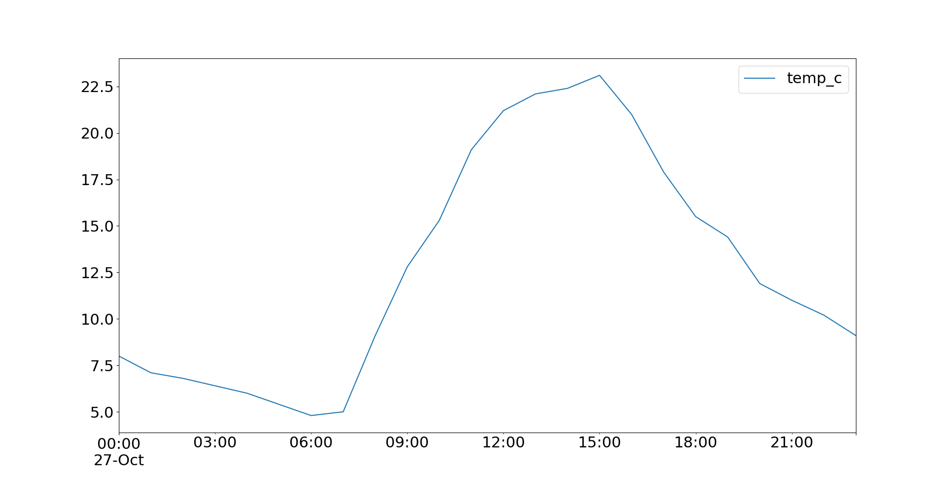
You can also apply .plot.line() and get the same result. Both .plot() and .plot.line() have many optional parameters that you can use to specify the look of your plot. Some of them are passed directly to the underlying Matplotlib methods.
You can save your figure by chaining the methods .get_figure() and .savefig():
>>> temp.plot().get_figure().savefig('temperatures.png')
This statement creates the plot and saves it as a file called 'temperatures.png' in your working directory.
You can get other types of plots with a pandas DataFrame. For example, you can visualize your job candidate data from before as a histogram with .plot.hist():
>>> df.loc[:, ['py-score', 'total']].plot.hist(bins=5, alpha=0.4)
<matplotlib.axes._subplots.AxesSubplot object at 0x7f070c69edd0>
>>> plt.show()
In this example, you extract the Python test score and total score data and visualize it with a histogram. The resulting plot looks like this:
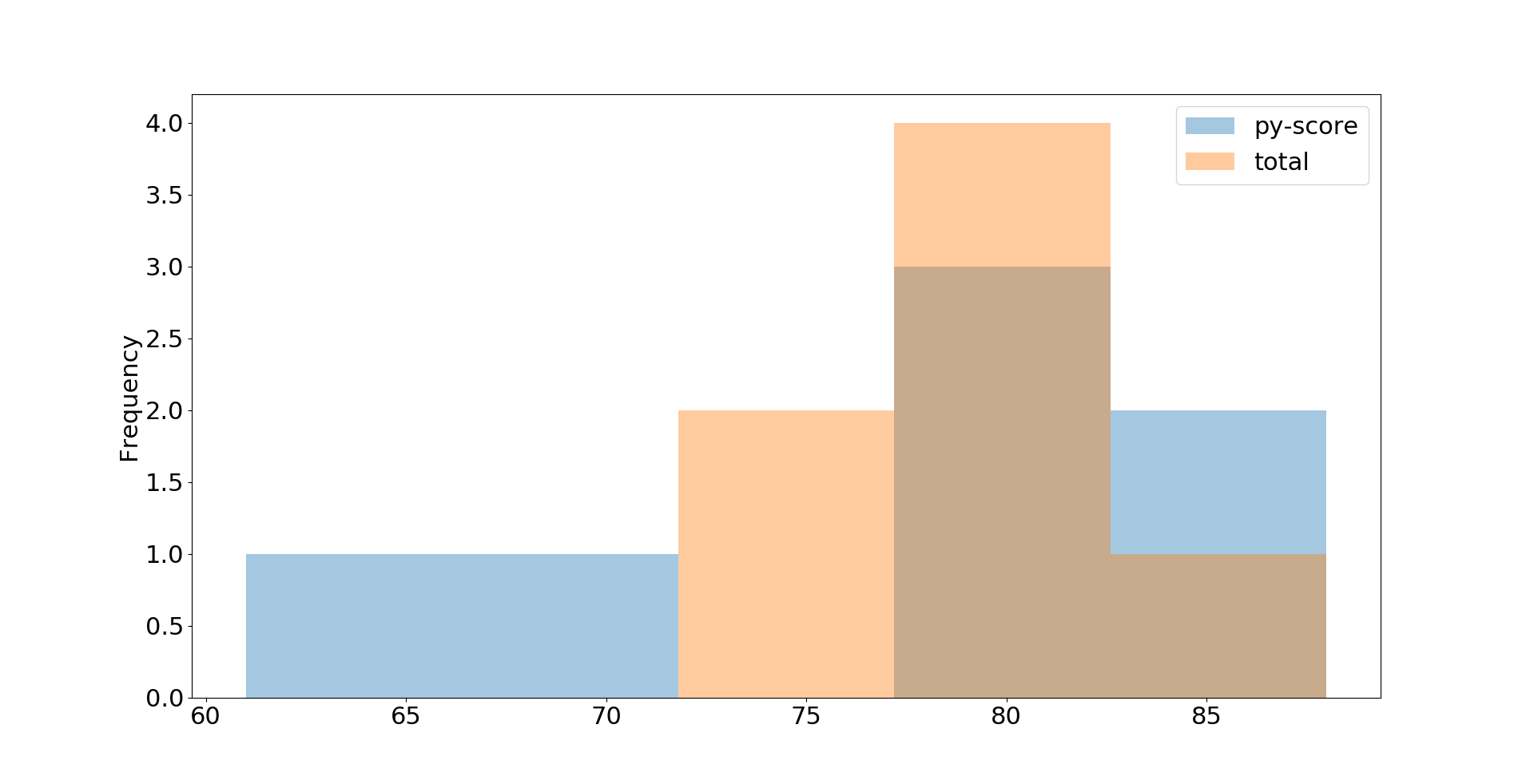
This is just the basic look. You can adjust details with optional parameters including .plot.hist(), Matplotlib’s plt.rcParams, and many others. You can find detailed explanations in the Anatomy of Matplotlib.
Further Reading
pandas DataFrames are very comprehensive objects that support many operations not mentioned in this tutorial. Some of these include:
- Hierarchical (multi-level) indexing
- Grouping
- Merging, joining, and concatenating
- Working with categorical data
The official pandas tutorial summarizes some of the available options nicely. If you want to learn more about pandas and DataFrames, then you can check out these tutorials:
- Pythonic Data Cleaning With pandas and NumPy
- pandas DataFrames 101
- Explore Your Dataset With pandas
- Python pandas: Tricks & Features You May Not Know
- Idiomatic pandas: Tricks & Features You May Not Know
- Reading CSVs With pandas
- Writing CSVs With pandas
- Reading and Writing CSV Files in Python
- Reading and Writing CSV Files
- Using pandas to Read Large Excel Files in Python
- Fast, Flexible, Easy and Intuitive: How to Speed Up Your pandas Projects
You’ve learned that pandas DataFrames handle two-dimensional data. If you need to work with labeled data in more than two dimensions, you can check out xarray, another powerful Python library for data science with very similar features to pandas.
If you work with big data and want a DataFrame-like experience, then you might give Dask a chance and use its DataFrame API. A Dask DataFrame contains many pandas DataFrames and performs computations in a lazy manner.
Conclusion
You now know what a pandas DataFrame is, what some of its features are, and how you can use it to work with data efficiently. pandas DataFrames are powerful, user-friendly data structures that you can use to gain deeper insight into your datasets!
In this tutorial, you’ve learned:
- What a pandas DataFrame is and how to create one
- How to access, modify, add, sort, filter, and delete data
- How to use NumPy routines with DataFrames
- How to handle missing values
- How to work with time-series data
- How to visualize data contained in DataFrames
You’ve learned enough to cover the fundamentals of DataFrames. If you want to dig deeper into working with data in Python, then check out the entire range of pandas tutorials.
If you have questions or comments, then please put them in the comment section below.
Take the Quiz: Test your knowledge with our interactive “The pandas DataFrame: Make Working With Data Delightful” quiz. You’ll receive a score upon completion to help you track your learning progress:
Interactive Quiz
The pandas DataFrame: Make Working With Data DelightfulTest your pandas skills! Practice DataFrame basics, column access, creation, sorting, and data manipulation in this interactive quiz.