If you’re familiar with functions in Python, then you know that it’s quite common for one function to call another. In Python, it’s also possible for a function to call itself! A function that calls itself is said to be recursive, and the technique of employing a recursive function is called recursion.
It may seem peculiar for a function to call itself, but many types of programming problems are best expressed recursively. When you bump up against such a problem, recursion is an indispensable tool for you to have in your toolkit.
Take the Quiz: Test your knowledge with our interactive “Recursion in Python: An Introduction” quiz. You’ll receive a score upon completion to help you track your learning progress:
Interactive Quiz
Recursion in Python: An IntroductionTest your understanding of recursion in Python, including base cases, recursive structure, performance considerations, and common use cases.
By the end of this tutorial, you’ll understand:
- What it means for a function to call itself recursively
- How the design of Python functions supports recursion
- What factors to consider when choosing whether or not to solve a problem recursively
- How to implement a recursive function in Python
Then you’ll study several Python programming problems that use recursion and contrast the recursive solution with a comparable non-recursive one.
Free Bonus: Get a sample chapter from Python Basics: A Practical Introduction to Python 3 to see how you can go from beginner to intermediate in Python with a complete curriculum, up to date for Python 3.9.
What Is Recursion?
The word recursion comes from the Latin word recurrere, meaning to run or hasten back, return, revert, or recur. Here are some online definitions of recursion:
- Dictionary.com: The act or process of returning or running back
- Wiktionary: The act of defining an object (usually a function) in terms of that object itself
- The Free Dictionary: A method of defining a sequence of objects, such as an expression, function, or set, where some number of initial objects are given and each successive object is defined in terms of the preceding objects
A recursive definition is one in which the defined term appears in the definition itself. Self-referential situations often crop up in real life, even if they aren’t immediately recognizable as such. For example, suppose you wanted to describe the set of people that make up your ancestors. You could describe them this way:

Notice how the concept that is being defined, ancestors, shows up in its own definition. This is a recursive definition.
In programming, recursion has a very precise meaning. It refers to a coding technique in which a function calls itself.
Why Use Recursion?
Most programming problems are solvable without recursion. So, strictly speaking, recursion usually isn’t necessary.
However, some situations particularly lend themselves to a self-referential definition—for example, the definition of ancestors shown above. If you were devising an algorithm to handle such a case programmatically, a recursive solution would likely be cleaner and more concise.
Traversal of tree-like data structures is another good example. Because these are nested structures, they readily fit a recursive definition. A non-recursive algorithm to walk through a nested structure is likely to be somewhat clunky, while a recursive solution will be relatively elegant. An example of this appears later in this tutorial.
On the other hand, recursion isn’t for every situation. Here are some other factors to consider:
- For some problems, a recursive solution, though possible, will be awkward rather than elegant.
- Recursive implementations often consume more memory than non-recursive ones.
- In some cases, using recursion may result in slower execution time.
Typically, the readability of the code will be the biggest determining factor. But it depends on the circumstances. The examples presented below should help you get a feel for when you should choose recursion.
Recursion in Python
When you call a function in Python, the interpreter creates a new local namespace so that names defined within that function don’t collide with identical names defined elsewhere. One function can call another, and even if they both define objects with the same name, it all works out fine because those objects exist in separate namespaces.
The same holds true if multiple instances of the same function are running concurrently. For example, consider the following definition:
def function():
    x = 10
    function()
When function() executes the first time, Python creates a namespace and assigns x the value 10 in that namespace. Then function() calls itself recursively. The second time function() runs, the interpreter creates a second namespace and assigns 10 to x there as well. These two instances of the name x are distinct from each another and can coexist without clashing because they are in separate namespaces.
Unfortunately, running function() as it stands produces a result that is less than inspiring, as the following traceback shows:
>>> function()
Traceback (most recent call last):
  File "<stdin>", line 1, in <module>
  File "<stdin>", line 3, in function
  File "<stdin>", line 3, in function
  File "<stdin>", line 3, in function
  [Previous line repeated 996 more times]
RecursionError: maximum recursion depth exceeded
As written, function() would in theory go on forever, calling itself over and over without any of the calls ever returning. In practice, of course, nothing is truly forever. Your computer only has so much memory, and it would run out eventually.
Python doesn’t allow that to happen. The interpreter limits the maximum number of times a function can call itself recursively, and when it reaches that limit, it raises a RecursionError exception, as you see above.
Technical note: You can find out what Python’s recursion limit is with a function from the sys module called getrecursionlimit():
>>> from sys import getrecursionlimit
>>> getrecursionlimit()
1000
You can change it, too, with setrecursionlimit():
>>> from sys import setrecursionlimit
>>> setrecursionlimit(2000)
>>> getrecursionlimit()
2000
You can set it to be pretty large, but you can’t make it infinite.
There isn’t much use for a function to indiscriminately call itself recursively without end. It’s reminiscent of the instructions that you sometimes find on shampoo bottles: “Lather, rinse, repeat.” If you were to follow these instructions literally, you’d shampoo your hair forever!
This logical flaw has evidently occurred to some shampoo manufacturers, because some shampoo bottles instead say “Lather, rinse, repeat as necessary.” That provides a termination condition to the instructions. Presumably, you’ll eventually feel your hair is sufficiently clean to consider additional repetitions unnecessary. Shampooing can then stop.
Similarly, a function that calls itself recursively must have a plan to eventually stop. Recursive functions typically follow this pattern:
- There are one or more base cases that are directly solvable without the need for further recursion.
- Each recursive call moves the solution progressively closer to a base case.
You’re now ready to see how this works with some examples.
Get Started: Count Down to Zero
The first example is a function called countdown(), which takes a positive number as an argument and prints the numbers from the specified argument down to zero:
>>> def countdown(n):
...     print(n)
...     if n == 0:
...         return             # Terminate recursion
...     else:
...         countdown(n - 1)   # Recursive call
...

>>> countdown(5)
5
4
3
2
1
0
Notice how countdown() fits the paradigm for a recursive algorithm described above:
- The base case occurs when
nis zero, at which point recursion stops. - In the recursive call, the argument is one less than the current value of
n, so each recursion moves closer to the base case.
Note: For simplicity, countdown() doesn’t check its argument for validity. If n is either a non-integer or negative, you’ll get a RecursionError exception because the base case is never reached.
The version of countdown() shown above clearly highlights the base case and the recursive call, but there’s a more concise way to express it:
def countdown(n):
    print(n)
    if n > 0:
        countdown(n - 1)
Here’s one possible non-recursive implementation for comparison:
>>> def countdown(n):
...     while n >= 0:
...         print(n)
...         n -= 1
...

>>> countdown(5)
5
4
3
2
1
0
This is a case where the non-recursive solution is at least as clear and intuitive as the recursive one, and probably more so.
Calculate Factorial
The next example involves the mathematical concept of factorial. The factorial of a positive integer n, denoted as n!, is defined as follows:

In other words, n! is the product of all integers from 1 to n, inclusive.
Factorial so lends itself to recursive definition that programming texts nearly always include it as one of the first examples. You can express the definition of n! recursively like this:

As with the example shown above, there are base cases that are solvable without recursion. The more complicated cases are reductive, meaning that they reduce to one of the base cases:
- The base cases (n = 0 or n = 1) are solvable without recursion.
- For values of n greater than 1, n! is defined in terms of (n - 1)!, so the recursive solution progressively approaches the base case.
For example, recursive computation of 4! looks like this:
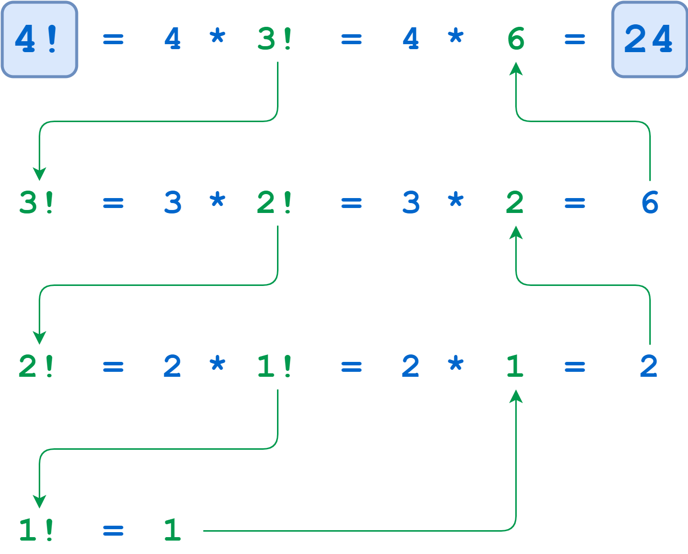
The calculations of 4!, 3!, and 2! suspend until the algorithm reaches the base case where n = 1. At that point, 1! is computable without further recursion, and the deferred calculations run to completion.
Define a Python Factorial Function
Here’s a recursive Python function to calculate factorial. Note how concise it is and how well it mirrors the definition shown above:
>>> def factorial(n):
...     return 1 if n <= 1 else n * factorial(n - 1)
...

>>> factorial(4)
24
A little embellishment of this function with some print() statements gives a clearer idea of the call and return sequence:
>>> def factorial(n):
...     print(f"factorial() called with n = {n}")
...     return_value = 1 if n <= 1 else n * factorial(n -1)
...     print(f"-> factorial({n}) returns {return_value}")
...     return return_value
...

>>> factorial(4)
factorial() called with n = 4
factorial() called with n = 3
factorial() called with n = 2
factorial() called with n = 1
-> factorial(1) returns 1
-> factorial(2) returns 2
-> factorial(3) returns 6
-> factorial(4) returns 24
24
Notice how all the recursive calls stack up. The function gets called with n = 4, 3, 2, and 1 in succession before any of the calls return. Finally, when n is 1, the problem can be solved without any more recursion. Then each of the stacked-up recursive calls unwinds back out, returning 1, 2, 6, and finally 24 from the outermost call.
Recursion isn’t necessary here. You could implement factorial() iteratively using a for loop:
>>> def factorial(n):
...     return_value = 1
...     for i in range(2, n + 1):
...         return_value *= i
...     return return_value
...

>>> factorial(4)
24
You can also implement factorial using Python’s reduce(), which you can import from the functools module:
>>> from functools import reduce
>>> def factorial(n):
...     return reduce(lambda x, y: x * y, range(1, n + 1) or [1])
...

>>> factorial(4)
24
Again, this shows that if a problem is solvable with recursion, there will also likely be several viable non-recursive solutions as well. You’ll typically choose based on which one results in the most readable and intuitive code.
Another factor to take into consideration is execution speed. There can be significant performance differences between recursive and non-recursive solutions. In the next section, you’ll explore these differences a little further.
Speed Comparison of Factorial Implementations
To evaluate execution time, you can use a function called timeit() from a module that is also called timeit. This function supports a number of different formats, but you’ll use the following format in this tutorial:
timeit(<command>, setup=<setup_string>, number=<iterations>)
timeit() first executes the commands contained in the specified <setup_string>. Then it executes <command> the given number of <iterations> and reports the cumulative execution time in seconds:
>>> from timeit import timeit

>>> timeit("print(string)", setup="string='foobar'", number=100)
foobar
foobar
foobar
   .
   . [100 repetitions]
   .
foobar
0.03347089999988384
Here, the setup parameter assigns string the value 'foobar'. Then timeit() prints string one hundred times. The total execution time is just over 3/100 of a second.
The examples shown below use timeit() to compare the recursive, iterative, and reduce() implementations of factorial from above. In each case, setup_string contains a setup string that defines the relevant factorial() function. timeit() then executes factorial(4) a total of ten million times and reports the aggregate execution.
First, here’s the recursive version:
>>> setup_string = """
... print("Recursive:")
... def factorial(n):
...     return 1 if n <= 1 else n * factorial(n - 1)
... """

>>> from timeit import timeit
>>> timeit("factorial(4)", setup=setup_string, number=10000000)
Recursive:
4.957105500000125
Next up is the iterative implementation:
>>> setup_string = """
... print("Iterative:")
... def factorial(n):
...     return_value = 1
...     for i in range(2, n + 1):
...         return_value *= i
...     return return_value
... """

>>> from timeit import timeit
>>> timeit("factorial(4)", setup=setup_string, number=10000000)
Iterative:
3.733752099999947
Last, here’s the version that uses reduce():
>>> setup_string = """
... from functools import reduce
... print("reduce():")
... def factorial(n):
...     return reduce(lambda x, y: x * y, range(1, n + 1) or [1])
... """

>>> from timeit import timeit
>>> timeit("factorial(4)", setup=setup_string, number=10000000)
reduce():
8.101526299999932
In this case, the iterative implementation is the fastest, although the recursive solution isn’t far behind. The method using reduce() is the slowest. Your mileage will probably vary if you try these examples on your own machine. You certainly won’t get the same times, and you may not even get the same ranking.
Does it matter? There’s a difference of almost four seconds in execution time between the iterative implementation and the one that uses reduce(), but it took ten million calls to see it.
If you’ll be calling a function many times, you might need to take execution speed into account when choosing an implementation. On the other hand, if the function will run relatively infrequently, then the difference in execution times will probably be negligible. In that case, you’d be better off choosing the implementation that seems to express the solution to the problem most clearly.
For factorial, the timings recorded above suggest a recursive implementation is a reasonable choice.
Frankly, if you’re coding in Python, you don’t need to implement a factorial function at all. It’s already available in the standard math module:
>>> from math import factorial
>>> factorial(4)
24
Perhaps it might interest you to know how this performs in the timing test:
>>> setup_string = "from math import factorial"

>>> from timeit import timeit
>>> timeit("factorial(4)", setup=setup_string, number=10000000)
0.3724050999999946
Wow! math.factorial() performs better than the best of the other three implementations shown above by roughly a factor of 10.
Technical note: The fact that math.factorial() is so much speedier probably has nothing to do with whether it’s implemented recursively. More likely it’s because the function is implemented in C rather than Python. For more reading on Python and C, see these resources:
A function implemented in C will virtually always be faster than a corresponding function implemented in pure Python.
Traverse a Nested List
The next example involves visiting each item in a nested list structure. Consider the following Python list:
names = [
    "Adam",
    [
        "Bob",
        [
            "Chet",
            "Cat",
        ],
        "Barb",
        "Bert"
    ],
    "Alex",
    [
        "Bea",
        "Bill"
    ],
    "Ann"
]
As the following diagram shows, names contains two sublists. The first of these sublists itself contains another sublist:
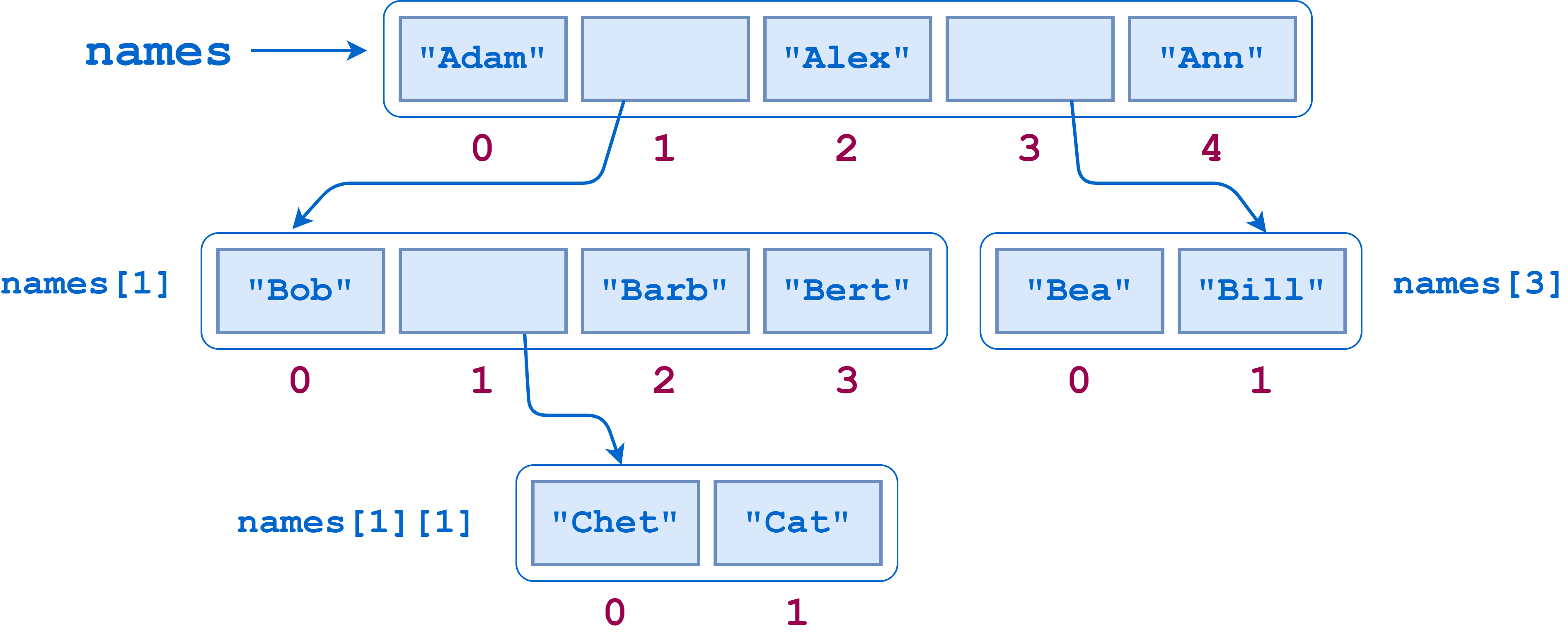
Suppose you wanted to count the number of leaf elements in this list—the lowest-level str objects—as though you’d flattened out the list. The leaf elements are "Adam", "Bob", "Chet", "Cat", "Barb", "Bert", "Alex", "Bea", "Bill", and "Ann", so the answer should be 10.
Just calling len() on the list doesn’t give the correct answer:
>>> len(names)
5
len() counts the objects at the top level of names, which are the three leaf elements "Adam", "Alex", and "Ann" and two sublists ["Bob", ["Chet", "Cat"], "Barb", "Bert"] and ["Bea", "Bill"]:
>>> for index, item in enumerate(names):
...     print(index, item)
...
0 Adam
1 ['Bob', ['Chet', 'Cat'], 'Barb', 'Bert']
2 Alex
3 ['Bea', 'Bill']
4 Ann
What you need here is a function that traverses the entire list structure, sublists included. The algorithm goes something like this:
- Walk through the list, examining each item in turn.
- If you find a leaf element, then add it to the accumulated count.
- If you encounter a sublist, then do the following:
- Drop down into that sublist and similarly walk through it.
- Once you’ve exhausted the sublist, go back up, add the elements from the sublist to the accumulated count, and resume the walk through the parent list where you left off.
Note the self-referential nature of this description: Walk through the list. If you encounter a sublist, then similarly walk through that list. This situation begs for recursion!
Traverse a Nested List Recursively
Recursion fits this problem very nicely. To solve it, you need to be able to determine whether a given list item is leaf item or not. For that, you can use the built-in Python function isinstance().
In the case of the names list, if an item is an instance of type list, then it’s a sublist. Otherwise, it’s a leaf item:
>>> names
['Adam', ['Bob', ['Chet', 'Cat'], 'Barb', 'Bert'], 'Alex', ['Bea', 'Bill'], 'Ann']

>>> names[0]
'Adam'
>>> isinstance(names[0], list)
False

>>> names[1]
['Bob', ['Chet', 'Cat'], 'Barb', 'Bert']
>>> isinstance(names[1], list)
True

>>> names[1][1]
['Chet', 'Cat']
>>> isinstance(names[1][1], list)
True

>>> names[1][1][0]
'Chet'
>>> isinstance(names[1][1][0], list)
False
Now you have the tools in place to implement a function that counts leaf elements in a list, accounting for sublists recursively:
def count_leaf_items(item_list):
    """Recursively counts and returns the
       number of leaf items in a (potentially
       nested) list.
    """
    count = 0
    for item in item_list:
        if isinstance(item, list):
            count += count_leaf_items(item)
        else:
            count += 1

    return count
If you run count_leaf_items() on several lists, including the names list defined above, you get this:
>>> count_leaf_items([1, 2, 3, 4])
4
>>> count_leaf_items([1, [2.1, 2.2], 3])
4
>>> count_leaf_items([])
0

>>> count_leaf_items(names)
10
>>> # Success!
As with the factorial example, adding some print() statements helps to demonstrate the sequence of recursive calls and return values:
 1def count_leaf_items(item_list):
 2    """Recursively counts and returns the
 3       number of leaf items in a (potentially
 4       nested) list.
 5    """
 6    print(f"List: {item_list}")
 7    count = 0
 8    for item in item_list:
 9        if isinstance(item, list):
10            print("Encountered sublist")
11            count += count_leaf_items(item)
12        else:
13            print(f"Counted leaf item \"{item}\"")
14            count += 1
15
16    print(f"-> Returning count {count}")
17    return count
Here’s a synopsis of what’s happening in the example above:
- Line 9:
isinstance(item, list)isTrue, socount_leaf_items()has found a sublist. - Line 11: The function calls itself recursively to count the items in the sublist, then adds the result to the accumulating total.
- Line 12:
isinstance(item, list)isFalse, socount_leaf_items()has encountered a leaf item. - Line 14: The function increments the accumulating total by one to account for the leaf item.
Note: To keep things simple, this implementation assumes the list passed to count_leaf_items() contains only leaf items or sublists, not any other type of composite object like a dictionary or tuple.
The output from count_leaf_items() when it’s executed on the names list now looks like this:
>>> count_leaf_items(names)
List: ['Adam', ['Bob', ['Chet', 'Cat'], 'Barb', 'Bert'], 'Alex', ['Bea', 'Bill'], 'Ann']
Counted leaf item "Adam"
Encountered sublist
List: ['Bob', ['Chet', 'Cat'], 'Barb', 'Bert']
Counted leaf item "Bob"
Encountered sublist
List: ['Chet', 'Cat']
Counted leaf item "Chet"
Counted leaf item "Cat"
-> Returning count 2
Counted leaf item "Barb"
Counted leaf item "Bert"
-> Returning count 5
Counted leaf item "Alex"
Encountered sublist
List: ['Bea', 'Bill']
Counted leaf item "Bea"
Counted leaf item "Bill"
-> Returning count 2
Counted leaf item "Ann"
-> Returning count 10
10
Each time a call to count_leaf_items() terminates, it returns the count of leaf elements it tallied in the list passed to it. The top-level call returns 10, as it should.
Traverse a Nested List Non-Recursively
Like the other examples shown so far, this list traversal doesn’t require recursion. You can also accomplish it iteratively. Here’s one possibility:
def count_leaf_items(item_list):
    """Non-recursively counts and returns the
       number of leaf items in a (potentially
       nested) list.
    """
    count = 0
    stack = []
    current_list = item_list
    i = 0

    while True:
        if i == len(current_list):
            if current_list == item_list:
                return count
            else:
                current_list, i = stack.pop()
                i += 1
                continue

        if isinstance(current_list[i], list):
            stack.append([current_list, i])
            current_list = current_list[i]
            i = 0
        else:
            count += 1
            i += 1
If you run this non-recursive version of count_leaf_items() on the same lists as shown previously, you get the same results:
>>> count_leaf_items([1, 2, 3, 4])
4
>>> count_leaf_items([1, [2.1, 2.2], 3])
4
>>> count_leaf_items([])
0

>>> count_leaf_items(names)
10
>>> # Success!
The strategy employed here uses a stack to handle the nested sublists. When this version of count_leaf_items() encounters a sublist, it pushes the list that is currently in progress and the current index in that list onto a stack. Once it has counted the sublist, the function pops the parent list and index from the stack so it can resume counting where it left off.
In fact, essentially the same thing happens in the recursive implementation as well. When you call a function recursively, Python saves the state of the executing instance on a stack so the recursive call can run. When the recursive call finishes, the state is popped from the stack so that the interrupted instance can resume. It’s the same concept, but with the recursive solution, Python is doing the state-saving work for you.
Notice how concise and readable the recursive code is when compared to the non-recursive version:
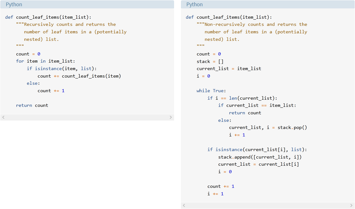
This is a case where using recursion is definitely an advantage.
Detect Palindromes
The choice of whether to use recursion to solve a problem depends in large part on the nature of the problem. Factorial, for example, naturally translates to a recursive implementation, but the iterative solution is quite straightforward as well. In that case, it’s arguably a toss-up.
The list traversal problem is a different story. In that case, the recursive solution is very elegant, while the non-recursive one is cumbersome at best.
For the next problem, using recursion is arguably silly.
A palindrome is a word that reads the same backward as it does forward. Examples include the following words:
- Racecar
- Level
- Kayak
- Reviver
- Civic
If asked to devise an algorithm to determine whether a string is palindromic, you would probably come up with something like “Reverse the string and see if it’s the same as the original.” You can’t get much plainer than that.
Even more helpfully, Python’s [::-1] slicing syntax for reversing a string provides a convenient way to code it:
>>> def is_palindrome(word):
...     """Return True if word is a palindrome, False if not."""
...     return word == word[::-1]
...

>>> is_palindrome("foo")
False
>>> is_palindrome("racecar")
True
>>> is_palindrome("troglodyte")
False
>>> is_palindrome("civic")
True
This is clear and concise. There’s hardly any need to look for an alternative. But just for fun, consider this recursive definition of a palindrome:
- Base cases: An empty string and a string consisting of a single character are inherently palindromic.
- Reductive recursion: A string of length two or greater is a palindrome if it satisfies both of these criteria:
- The first and last characters are the same.
- The substring between the first and last characters is a palindrome.
Slicing is your friend here as well. For a string word, indexing and slicing give the following substrings:
- The first character is
word[0]. - The last character is
word[-1]. - The substring between the first and last characters is
word[1:-1].
So you can define is_palindrome() recursively like this:
>>> def is_palindrome(word):
...     """Return True if word is a palindrome, False if not."""
...     if len(word) <= 1:
...         return True
...     else:
...         return word[0] == word[-1] and is_palindrome(word[1:-1])
...

>>> # Base cases
>>> is_palindrome("")
True
>>> is_palindrome("a")
True

>>> # Recursive cases
>>> is_palindrome("foo")
False
>>> is_palindrome("racecar")
True
>>> is_palindrome("troglodyte")
False
>>> is_palindrome("civic")
True
It’s an interesting exercise to think recursively, even when it isn’t especially necessary.
Sort With Quicksort
The final example presented, like the nested list traversal, is a good example of a problem that very naturally suggests a recursive approach. The Quicksort algorithm is an efficient sorting algorithm developed by British computer scientist Tony Hoare in 1959.
Quicksort is a divide-and-conquer algorithm. Suppose you have a list of objects to sort. You start by choosing an item in the list, called the pivot item. This can be any item in the list. You then partition the list into two sublists based on the pivot item and recursively sort the sublists.
The steps of the algorithm are as follows:
- Choose the pivot item.
- Partition the list into two sublists:
- Those items that are less than the pivot item
- Those items that are greater than the pivot item
- Quicksort the sublists recursively.
Each partitioning produces smaller sublists, so the algorithm is reductive. The base cases occur when the sublists are either empty or have one element, as these are inherently sorted.
Choosing the Pivot Item
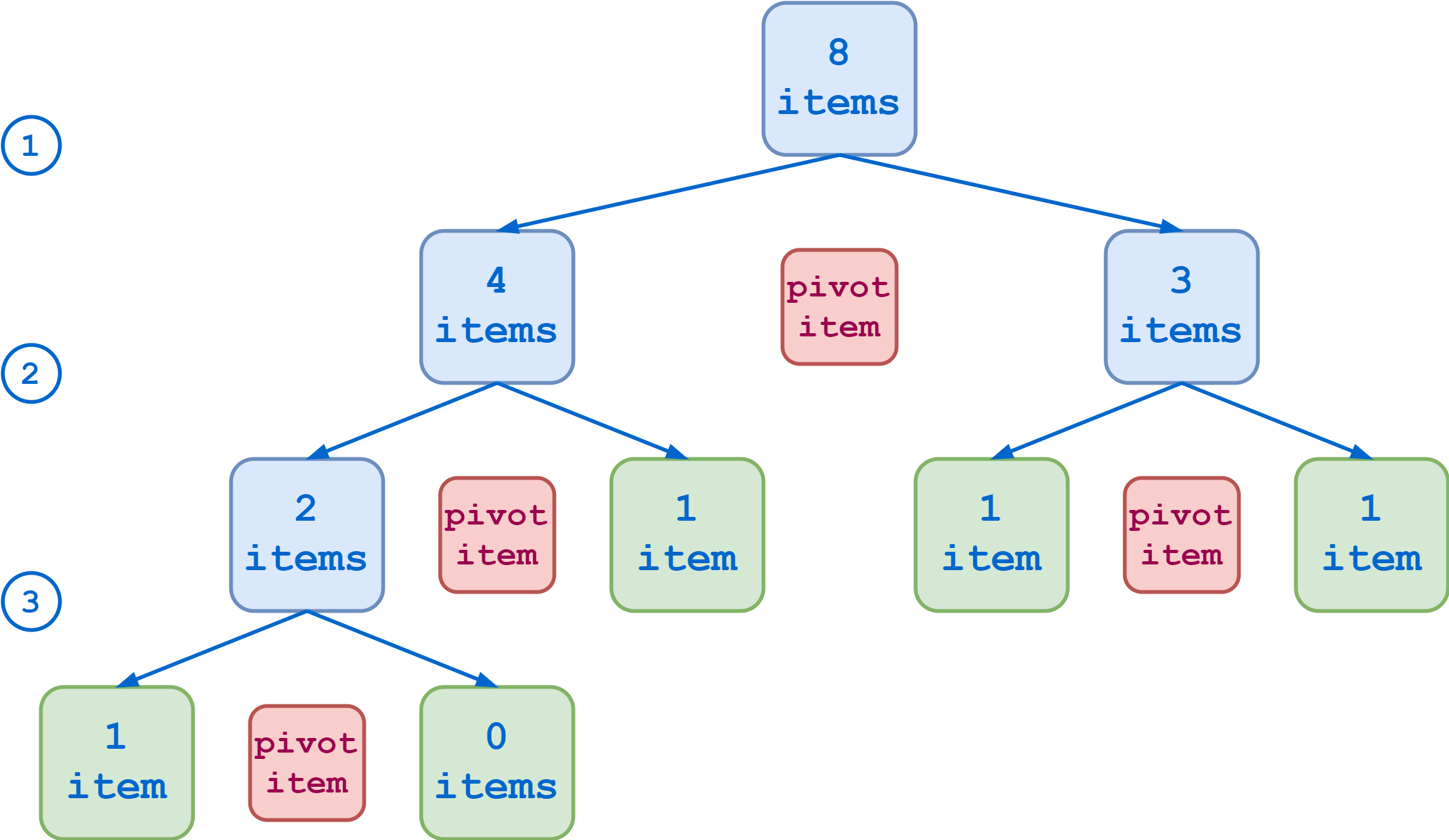
The Quicksort algorithm will work no matter what item in the list is the pivot item. But some choices are better than others. Remember that when partitioning, two sublists that are created: one with items that are less than the pivot item and one with items that are greater than the pivot item. Ideally, the two sublists are of roughly equal length.
Imagine that your initial list to sort contains eight items. If each partitioning results in sublists of roughly equal length, then you can reach the base cases in three steps:
At the other end of the spectrum, if your choice of pivot item is especially unlucky, each partition results in one sublist that contains all the original items except the pivot item and another sublist that is empty. In that case, it takes seven steps to reduce the list to the base cases:
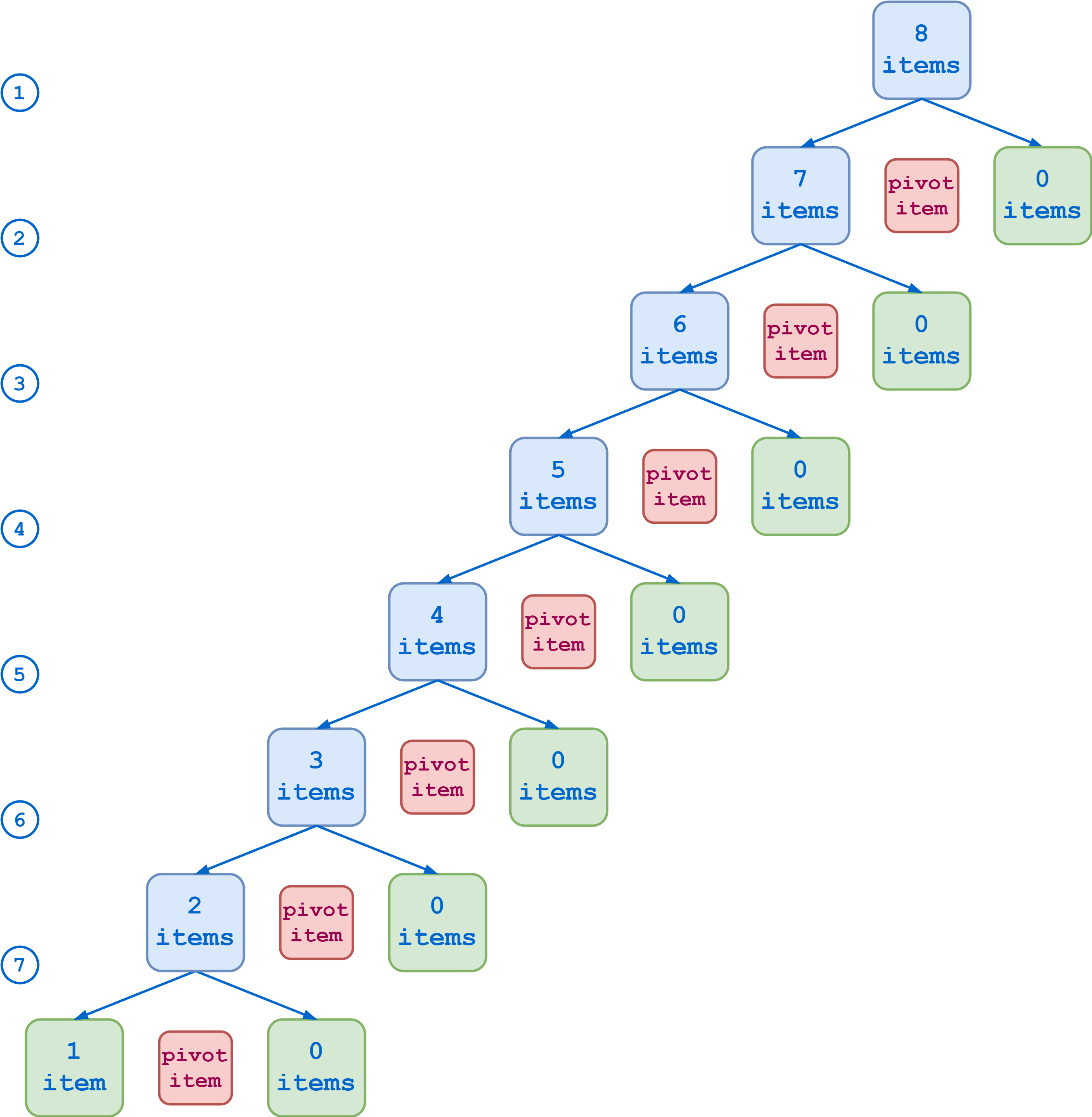
The Quicksort algorithm will be more efficient in the first case. But you’d need to know something in advance about the nature of the data you’re sorting in order to systematically choose optimal pivot items. In any case, there isn’t any one choice that will be the best for all cases. So if you’re writing a Quicksort function to handle the general case, the choice of pivot item is somewhat arbitrary.
The first item in the list is a common choice, as is the last item. These will work fine if the data in the list is fairly randomly distributed. However, if the data is already sorted, or even nearly so, then these will result in suboptimal partitioning like that shown above. To avoid this, some Quicksort algorithms choose the middle item in the list as the pivot item.
Another option is to find the median of the first, last, and middle items in the list and use that as the pivot item. This is the strategy used in the sample code below.
Implementing the Partitioning
Once you’ve chosen the pivot item, the next step is to partition the list. Again, the goal is to create two sublists, one containing the items that are less than the pivot item and the other containing those that are greater.
You could accomplish this directly in place. In other words, by swapping items, you could shuffle the items in the list around until the pivot item is in the middle, all the lesser items are to its left, and all the greater items are to its right. Then, when you Quicksort the sublists recursively, you’d pass the slices of the list to the left and right of the pivot item.
Alternately, you can use Python’s list manipulation capability to create new lists instead of operating on the original list in place. This is the approach taken in the code below. The algorithm is as follows:
- Choose the pivot item using the median-of-three method described above.
- Using the pivot item, create three sublists:
- The items in the original list that are less than the pivot item
- The pivot item itself
- The items in the original list that are greater than the pivot item
- Recursively Quicksort lists 1 and 3.
- Concatenate all three lists back together.
Note that this involves creating a third sublist that contains the pivot item itself. One advantage to this approach is that it smoothly handles the case where the pivot item appears in the list more than once. In that case, list 2 will have more than one element.
Using the Quicksort Implementation
Now that the groundwork is in place, you are ready to move on to the Quicksort algorithm. Here’s the Python code:
 1import statistics
 2
 3def quicksort(numbers):
 4    if len(numbers) <= 1:
 5        return numbers
 6    else:
 7        pivot = statistics.median(
 8            [
 9                numbers[0],
10                numbers[len(numbers) // 2],
11                numbers[-1]
12            ]
13        )
14        items_less, pivot_items, items_greater = (
15            [n for n in numbers if n < pivot],
16            [n for n in numbers if n == pivot],
17            [n for n in numbers if n > pivot]
18        )
19
20        return (
21            quicksort(items_less) +
22            pivot_items +
23            quicksort(items_greater)
24        )
This is what each section of quicksort() is doing:
- Line 4: The base cases where the list is either empty or has only a single element
- Lines 7 to 13: Calculation of the pivot item by the median-of-three method
- Lines 14 to 18: Creation of the three partition lists
- Lines 20 to 24: Recursive sorting and reassembly of the partition lists
Note: This example has the advantage of being succinct and relatively readable. However, it isn’t the most efficient implementation. In particular, the creation of the partition lists on lines 14 to 18 involves iterating through the list three separate times, which isn’t optimal from the standpoint of execution time.
Here are some examples of quicksort() in action:
>>> # Base cases
>>> quicksort([])
[]
>>> quicksort([42])
[42]

>>> # Recursive cases
>>> quicksort([5, 2, 6, 3])
[2, 3, 5, 6]
>>> quicksort([10, -3, 21, 6, -8])
[-8, -3, 6, 10, 21]
For testing purposes, you can define a short function that generates a list of random numbers between 1 and 100:
import random

def get_random_numbers(length, minimum=1, maximum=100):
    numbers = []
    for _ in range(length):
        numbers.append(random.randint(minimum, maximum))

    return numbers
Now you can use get_random_numbers() to test quicksort():
>>> numbers = get_random_numbers(20)
>>> numbers
[24, 4, 67, 71, 84, 63, 100, 94, 53, 64, 19, 89, 48, 7, 31, 3, 32, 76, 91, 78]
>>> quicksort(numbers)
[3, 4, 7, 19, 24, 31, 32, 48, 53, 63, 64, 67, 71, 76, 78, 84, 89, 91, 94, 100]

>>> numbers = get_random_numbers(15, -50, 50)
>>> numbers
[-2, 14, 48, 42, -48, 38, 44, -25, 14, -14, 41, -30, -35, 36, -5]
>>> quicksort(numbers)
[-48, -35, -30, -25, -14, -5, -2, 14, 14, 36, 38, 41, 42, 44, 48]

>>> quicksort(get_random_numbers(10, maximum=500))
[49, 94, 99, 124, 235, 287, 292, 333, 455, 464]
>>> quicksort(get_random_numbers(10, 1000, 2000))
[1038, 1321, 1530, 1630, 1835, 1873, 1900, 1931, 1936, 1943]
To further understand how quicksort() works, see the diagram below. This shows the recursion sequence when sorting a twelve-element list:
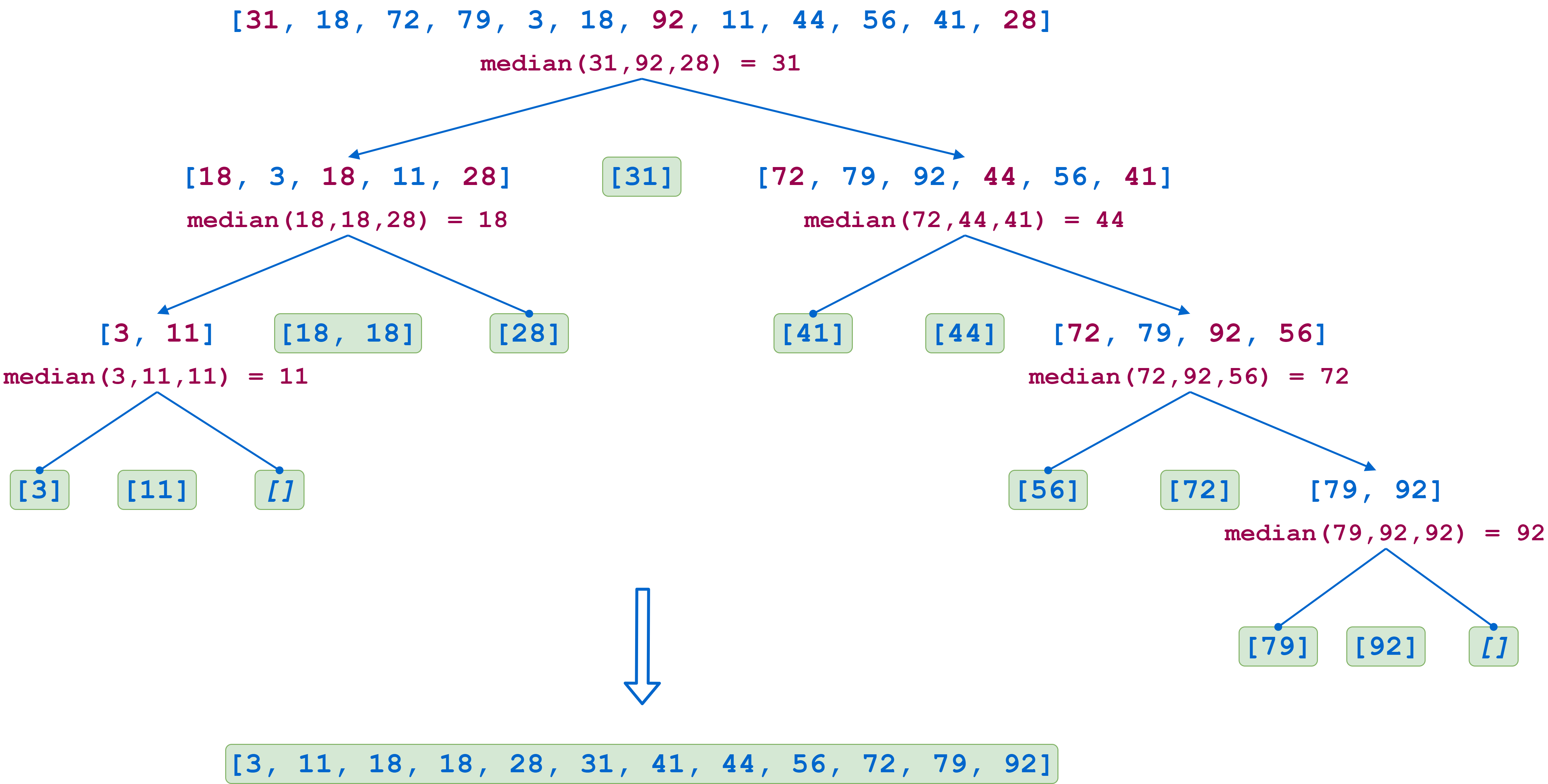
In the first step, the first, middle, and last list values are 31, 92, and 28, respectively. The median is 31, so that becomes the pivot item. The first partition then consists of the following sublists:
| Sublist | Items |
|---|---|
[18, 3, 18, 11, 28] |
The items less than the pivot item |
[31] |
The pivot item itself |
[72, 79, 92, 44, 56, 41] |
The items greater than the pivot item |
Each sublist is subsequently partitioned recursively in the same manner until all the sublists either contain a single element or are empty. As the recursive calls return, the lists are reassembled in sorted order. Note that in the second-to-last step on the left, the pivot item 18 appears in the list twice, so the pivot item list has two elements.
Conclusion
That concludes your journey through recursion, a programming technique in which a function calls itself. Recursion isn’t by any means appropriate for every task. But some programming problems virtually cry out for it. In those situations, it’s a great technique to have at your disposal.
In this tutorial, you learned:
- What it means for a function to call itself recursively
- How the design of Python functions supports recursion
- What factors to consider when choosing whether or not to solve a problem recursively
- How to implement a recursive function in Python
You also saw several examples of recursive algorithms and compared them to corresponding non-recursive solutions.
You should now be in a good position to recognize when recursion is called for and be ready to use it confidently when it’s needed!
Work through the quiz questions to test your understanding and identify any gaps to review and practice:
Take the Quiz: Test your knowledge with our interactive “Recursion in Python: An Introduction” quiz. You’ll receive a score upon completion to help you track your learning progress:
Interactive Quiz
Recursion in Python: An IntroductionTest your understanding of recursion in Python, including base cases, recursive structure, performance considerations, and common use cases.
If you want to explore more about recursion in Python, then check out Thinking Recursively in Python.

