GeoPandas extends pandas to make working with geospatial data in Python intuitive and powerful. If you’re looking to do geospatial tasks in Python and want a library with a pandas-like API, then GeoPandas is an excellent choice. This tutorial shows you how to accomplish four common geospatial tasks: reading in data, mapping it, applying a projection, and doing a spatial join.
By the end of this tutorial, you’ll understand that:
- GeoPandas extends pandas with support for spatial data. This data typically lives in a
geometrycolumn and allows spatial operations such as projections and spatial joins, while Folium focuses on richer interactive web maps after data preparation. - You inspect CRS with
.crsand reproject data using.to_crs()with an authority code likeEPSG:4326orESRI:54009. - A geographic CRS stores longitude and latitude in degrees, while a projected CRS uses linear units like meters or feet for area and distance calculations.
- Spatial joins use
.sjoin()with predicates like"within"or"intersects", and both inputs must share the same CRS or the relationships will be computed incorrectly.
Here’s how GeoPandas compares with alternative libraries:
| Use Case | Pick pandas | Pick Folium | Pick GeoPandas |
|---|---|---|---|
| Tabular data analysis | ✅ | - | ✅ |
| Mapping | - | ✅ | ✅ |
| Projections, spatial joins | - | - | ✅ |
GeoPandas builds on pandas by adding support for geospatial data and operations like projections and spatial joins. It also includes tools for creating maps. Folium complements this by focusing on interactive, web-based maps that you can customize more deeply.
Get Your Code: Click here to download the free sample code for learning how to work with GeoPandas maps, projections, and spatial joins.
Take the Quiz: Test your knowledge with our interactive “GeoPandas Basics: Maps, Projections, and Spatial Joins” quiz. You’ll receive a score upon completion to help you track your learning progress:

Interactive Quiz
GeoPandas Basics: Maps, Projections, and Spatial JoinsTest GeoPandas basics for reading, mapping, projecting, and spatial joins to handle geospatial data confidently.
Getting Started With GeoPandas
You’ll first prepare your environment and load a small dataset that you’ll use throughout the tutorial. In the next two subsections, you’ll install the necessary packages and read in a sample dataset of New York City borough boundaries. This gives you a concrete GeoDataFrame to explore as you learn the core concepts.
Installing GeoPandas
This tutorial uses two packages: geopandas for working with geographic data and geodatasets for loading sample data. It’s a good idea to install these packages inside a virtual environment so your project stays isolated from the rest of your system and you can manage its dependencies cleanly.
Once your virtual environment is active, you can install both packages with pip:
$ python -m pip install "geopandas[all]" geodatasets
Using the [all] option ensures you have everything needed for reading data, transforming coordinate systems, and creating plots. For most readers, this will work out of the box.
If you do run into installation issues, the project’s maintainers provide alternative installation options on the official installation page.
Reading in Data
Most geospatial datasets come in GeoJSON or shapefile format. The read_file() function can read both, and it accepts either a local file path or a URL.
In the example below, you’ll use read_file() to load the New York City Borough Boundaries (NYBB) dataset. The geodatasets package provides a convenient path to this dataset, so you don’t need to download anything manually. You’ll also drop unnecessary columns:
>>> import geopandas as gpd
>>> import matplotlib.pyplot as plt
>>> from geodatasets import get_path
>>> path_to_data = get_path("nybb")
>>> nybb = gpd.read_file(path_to_data)
>>> nybb = nybb[["BoroName", "Shape_Area", "geometry"]]
>>> nybb
    BoroName        Shape_Area      geometry
0   Staten Island   1.623820e+09    MULTIPOLYGON (((970217.022 145643.332, ....
1   Queens          3.045213e+09    MULTIPOLYGON (((1029606.077 156073.814, ...
2   Brooklyn        1.937479e+09    MULTIPOLYGON (((1021176.479 151374.797, ...
3   Manhattan       6.364715e+08    MULTIPOLYGON (((981219.056 188655.316, ....
4   Bronx           1.186925e+09    MULTIPOLYGON (((1012821.806 229228.265, ...
>>> type(nybb)
<class 'geopandas.geodataframe.GeoDataFrame'>
>>> type(nybb["geometry"])
<class 'geopandas.geoseries.GeoSeries'>
nybb is a GeoDataFrame. A GeoDataFrame has rows, columns, and all the methods of a pandas DataFrame. The difference is that it typically includes a special geometry column, which stores geographic shapes instead of plain numbers or text.
The geometry column is a GeoSeries. It behaves like a normal pandas Series, but its values are spatial objects that you can map and run spatial queries against. In the nybb dataset, each borough’s geometry is a MultiPolygon—a shape made of several polygons—because every borough consists of multiple islands. Soon you’ll use these geometries to make maps and run spatial operations, such as finding which borough a point falls inside.
Mapping Data
Once you’ve loaded a GeoDataFrame, one of the quickest ways to understand your data is to visualize it. In this section, you’ll learn how to create both static and interactive maps. This allows you to inspect shapes, spot patterns, and confirm that your geometries look the way you expect.
Creating Static Maps
As explained in the guide to plotting with pandas, pandas DataFrames have a .plot() method for creating quick visualizations like scatter plots or bar charts. The GeoDataFrame class overrides .plot() so that, when your data contains geometry, the result is a map instead of a chart.
Here, you call nybb.plot() to draw the outlines of New York City’s five boroughs:
>>> nybb.plot()
<Axes: >
>>> plt.show()
The resulting image is:
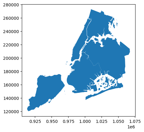
This kind of quick plot is useful for checking that your data loaded correctly and that the geometries look reasonable. But often you’ll want to go a step further and use color to show a value for each region. A map that colors areas based on values in a column is called a choropleth, and you can create one by passing the column you want to visualize to the column parameter:
>>> nybb.plot(column="Shape_Area", legend=True)
<Axes: >
>>> plt.show()
This gives the following output:
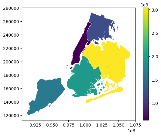
Here you can see the relative size of each borough expressed with color.
Creating Interactive Maps
You can also create interactive, zoomable maps using the .explore() method. Under the hood, .explore() uses the Folium library to generate an HTML map. The REPL can’t display it directly, and the .show_in_browser() method opens the map in your default browser:
>>> nybb.explore().show_in_browser()
This launches an interactive map in your browser. You should see something like this:
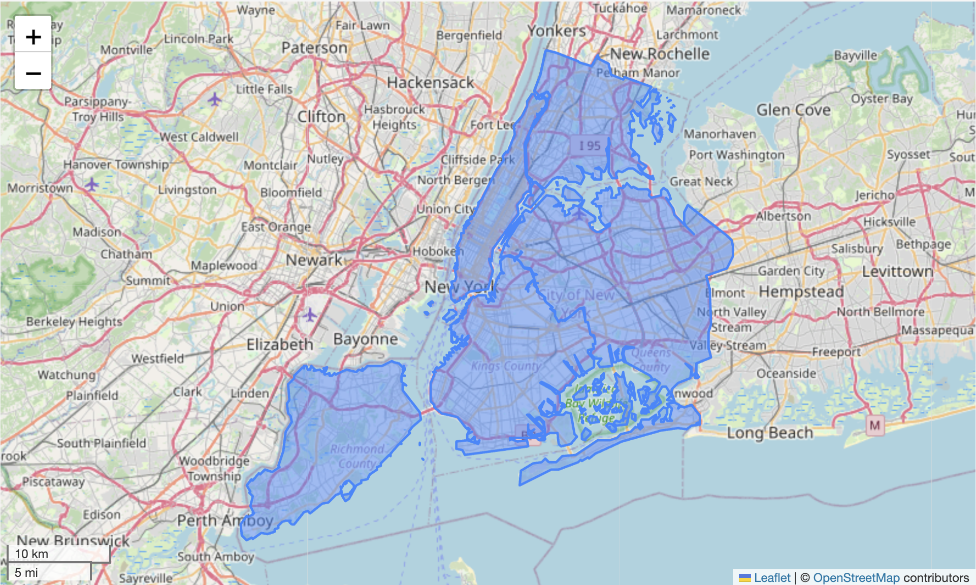
Unlike .plot(), which draws simple static shapes, .explore() overlays your data on a reference map—complete with place names, coastlines, and zoom controls. This makes it easier to interpret your data in context and explore the geography interactively.
Just like with .plot(), you can turn this into a choropleth by passing a column name. Here you color each borough by its land area:
>>> nybb.explore(column="Shape_Area", legend=False).show_in_browser()
The output is:
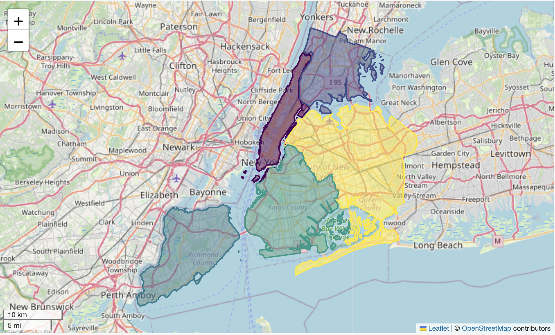
And now the relative size of each borough is expressed with color, giving you a sense of how interactive maps can reveal patterns in your data. To make these maps accurate and comparable across datasets, you’ll next look at how coordinate reference systems and projections work.
Working With Coordinate Reference Systems (CRS) and Projections
Every GeoDataFrame includes a Coordinate Reference System (CRS) that explains how its coordinates map to real-world locations. Understanding the CRS is essential for interpreting geometry values, comparing datasets, and producing accurate maps. Before exploring it further, take a closer look at the geometry column of nybb:
>>> nybb[["BoroName", "geometry"]]
     BoroName       geometry
0    Staten Island  MULTIPOLYGON (((970217.022 145643.332, 970227....
1    Queens         MULTIPOLYGON (((1029606.077 156073.814, 102957...
2    Brooklyn       MULTIPOLYGON (((1021176.479 151374.797, 102100...
3    Manhattan      MULTIPOLYGON (((981219.056 188655.316, 980940....
4    Bronx          MULTIPOLYGON (((1012821.806 229228.265, 101278...
Notice that the geometry column is just numbers—it’s not obvious how these values correspond to places on Earth.
The CRS for each GeoDataFrame is in its .crs attribute. Here’s the CRS of the nybb dataset:
>>> nybb.crs
<Projected CRS: EPSG:2263>
Name: NAD83 / New York Long Island (ftUS)
Axis Info [cartesian]:
- X[east]: Easting (US survey foot)
- Y[north]: Northing (US survey foot)
Area of Use:
- name: United States (USA) - New York - counties of Bronx; Kings; Nassau ...
- bounds: (-74.26, 40.47, -71.8, 41.3)
Coordinate Operation:
- name: SPCS83 New York Long Island zone (US survey foot)
- method: Lambert Conic Conformal (2SP)
Datum: North American Datum 1983
- Ellipsoid: GRS 1980
- Prime Meridian: Greenwich
Every CRS has both a name and a code. In this case, the CRS is called NAD83 / New York Long Island (ftUS) and its code is EPSG:2263. The x- and y-coordinates represent distances in US survey feet, and the origin sits far outside New York City. That placement explains the large axis values, since they show how many feet east and north each point is from that origin.
EPSG:2263 is a projected CRS. That means the coordinates in the geometry column have been transformed using a mathematical projection so that the x- and y-axes represent linear distances. In the next section, you’ll look at a geographic CRS, where the axes aren’t distances at all, but degrees of latitude and longitude.
Exploring Geographic CRS
A common CRS to use when looking at a world map is WGS 84 (EPSG:4326). Here’s how you can load a world map with this CRS:
>>> world = gpd.read_file(get_path("naturalearth land"))
>>> world.crs
<Geographic 2D CRS: EPSG:4326>
Name: WGS 84
Axis Info [ellipsoidal]:
- Lat[north]: Geodetic latitude (degree)
- Lon[east]: Geodetic longitude (degree)
Area of Use:
- name: World.
- bounds: (-180.0, -90.0, 180.0, 90.0)
Datum: World Geodetic System 1984 ensemble
- Ellipsoid: WGS 84
- Prime Meridian: Greenwich
WGS 84 is a geographic CRS: the x- and y-axes represent longitude and latitude in degrees. They don’t represent physical distances like feet or meters. Since degrees aren’t uniform distances, plotting a geographic CRS directly distorts shapes and areas, especially at the poles.
Here’s how to plot the world map:
>>> world.plot()
<Axes: >
>>> plt.show()
And here’s the result:
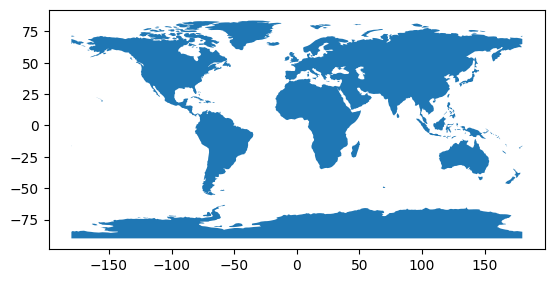
Because this CRS isn’t projected, areas near the poles appear stretched—Greenland and Antarctica look much larger than they actually are.
Changing CRS
You can change the CRS of a GeoDataFrame. This matters because the choice of CRS affects how distances, areas, and shapes appear.
For example, you just saw that WGS 84 makes Greenland and Antarctica appear much larger than they are. The Mollweide projection is an equal-area projection: every region preserves its true proportion of area relative to every other region. Shapes become more rounded, and distances vary, but the relative sizes of continents and countries are accurate.
You can change the CRS of the world map from WGS 84 to Mollweide with the method .to_crs():
>>> world_moll = world.to_crs("ESRI:54009")
>>> world_moll.crs
<Projected CRS: ESRI:54009>
Name: World_Mollweide
Axis Info [cartesian]:
- E[east]: Easting (metre)
- N[north]: Northing (metre)
Area of Use:
- name: World.
- bounds: (-180.0, -90.0, 180.0, 90.0)
Coordinate Operation:
- name: World_Mollweide
- method: Mollweide
Datum: World Geodetic System 1984
- Ellipsoid: WGS 84
- Prime Meridian: Greenwich
As with all projected CRS, the axes of the map are in distances, not degrees of latitude and longitude.
You can plot the world map with the new CRS like this:
>>> world_moll.plot()
<Axes: >
>>> plt.show()
The output looks as follows:
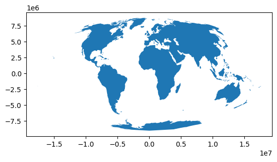
In this map, Greenland and Antarctica appear much smaller than in the WGS 84 plot. More importantly, their size is accurate in comparison to other landmasses.
Comparing CRS
Sometimes it’s helpful to do a side-by-side comparison of a dataset under two different CRS. This example, which uses Matplotlib, plots the same world map using both WGS 84 and Mollweide:
>>> fig, axes = plt.subplots(1, 2, figsize=(14, 7))
>>> world.plot(ax=axes[0])
<Axes: >
>>> axes[0].set_title("EPSG:4326 (WGS84 Lat/Lon)")
Text(0.5, 1.0, 'EPSG:4326 (WGS84 Lat/Lon)')
>>> world_moll.plot(ax=axes[1])
<Axes: >
>>> axes[1].set_title("ESRI:54009 (Mollweide Equal-Area)")
Text(0.5, 1.0, 'ESRI:54009 (Mollweide Equal-Area)')
>>> plt.tight_layout()
>>> plt.show()
This is how the final comparison image looks:
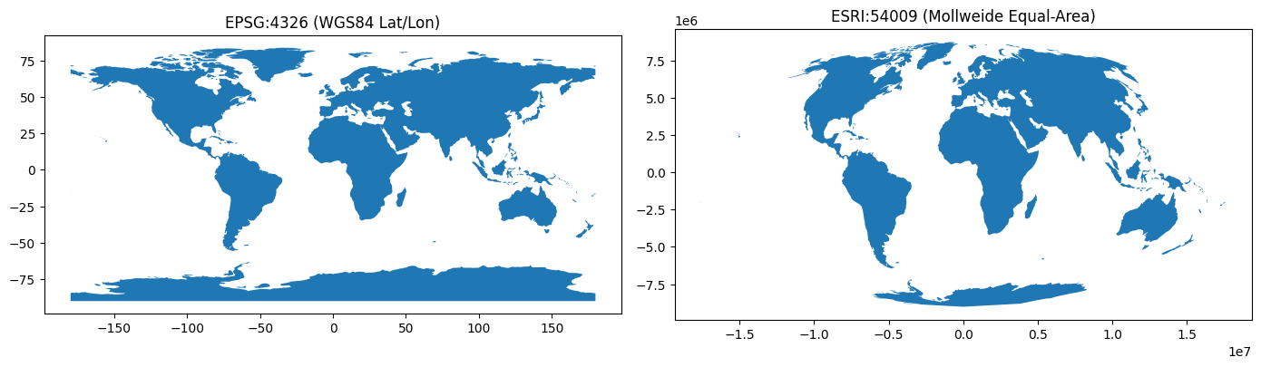
In this plot, it’s clear that the choice of CRS impacts the way the map is rendered. Because WGS 84 treats longitude and latitude as x- and y-coordinates, areas near the poles appear stretched and larger than they really are. By contrast, the Mollweide projection preserves the relative size of each landmass, so Greenland and Antarctica appear much smaller.
Understanding Map Projections and CRS
As you’ve seen, GeoPandas uses Coordinate Reference Systems (CRS) to map coordinates to real-world locations. Some CRS are geographic and use latitude and longitude in degrees. These aren’t projected. Others are projected, meaning they use a map projection to flatten the Earth into x- and y-coordinates in linear units.
Every projection is part of a CRS, but not every CRS uses a projection.
Performing Spatial Joins
A spatial join lets you combine information from two GeoDataFrames based on how their geometries relate to each other. Instead of matching rows by a shared ID or column name, a spatial join matches features by where they are in space—for example, which subway stations are within a borough. It’s the geospatial equivalent of a database join, but the key is location rather than a field value.
In the example below, you use a spatial join to see which borough of New York City contains the Empire State Building. Start by creating a GeoDataFrame with the longitude and latitude of the Empire State Building. Because these coordinates are expressed in degrees, you should use EPSG:4326 for the CRS:
>>> from shapely.geometry import Point
>>> empire_state = gpd.GeoDataFrame(
...    [{"name": "Empire State Building"}],
...    geometry=[Point(-73.9857, 40.7484)],
...    crs="EPSG:4326"
... )
>>> empire_state
     name                     geometry
0    Empire State Building    POINT (-73.9857 40.7484)
You now have a GeoDataFrame with exactly one point.
Understanding Spatial Joins and CRS
Spatial joins require the two GeoDataFrames to have the same CRS. You just saw that the empire_state DataFrame uses EPSG:4326. Earlier, you saw that nybb uses EPSG:2263. Here’s how you can change empire_state to also use EPSG:2263:
>>> empire_state = empire_state.to_crs(nybb.crs)
>>> empire_state
     name                     geometry
0    Empire State Building    POINT (988212.237 211939.279)
Note that when you changed the CRS of empire_state, the values in the geometry column changed from (-73.9857, 40.7484) to (988212.237, 211939.279). This is because coordinates only have meaning within the context of a CRS. When you switch to a different CRS, the same real-world location is expressed with different coordinate values.
Using the .sjoin() Method
Spatial joins in GeoPandas work similarly to how joins in pandas work. Namely, GeoDataFrames have a .sjoin() instance method. This method requires you to specify a GeoDataFrame to join with, as well as which type of join and predicate to use.
In the example below, you join the empire_state DataFrame to the nybb DataFrame using a left join. With a left join, you’re guaranteed to get back at least one row, which will be the row from the original empire_state DataFrame.
Before running the join, it’s important to understand how the predicate parameter works. The predicate parameter tells .sjoin() how to decide whether two geometries match spatially. Here, you use "within" because you want to test whether a point is within a borough:
>>> empire_state.sjoin(nybb, how="left", predicate="within")
   name                   geometry               index_right  BoroName  ...
0  Empire State Building  POINT (988212.237 ...  3            Manhattan ...
You only get one row back because the New York City boroughs don’t overlap. The Empire State Building is in Manhattan, which is what the join shows. Since you joined the two DataFrames, you have columns from both empire_state and nybb.
In this example, you looked at the "within" predicate, which lets you test whether one shape is within another. Other predicates let you test whether two shapes touch, overlap, intersect, and so on.
Avoiding Limitations and Gotchas
Even though GeoPandas is powerful and beginner-friendly, there are a few common pitfalls that can trip people up—especially when you start working with real-world data.
Keeping these in mind will save you time and confusion:
- Dependencies: Installing GeoPandas can be tricky because it depends on compiled libraries (
GEOS,PROJ,GDAL). If you run into problems installing withpip, see the official installation page for information about alternatives. - CRS awareness: Always check and set the CRS. Forgetting to reproject before spatial joins or distance calculations can lead to incorrect results.
- Mapping limits:
.plot()and.explore()are great for quick maps, but customization is limited. For advanced interactivity such as multiple layers, popups, and basemaps, you’ll want to use Folium directly.
These aren’t deal-breakers—just patterns worth recognizing early so your workflow stays smooth and predictable.
Conclusion
GeoPandas extends the familiar pandas workflow into the geospatial world. Along the way, you learned how to load common geospatial formats, create both static and interactive maps, work with and change a dataset’s CRS, and use spatial joins to answer location-based questions.
You now have the core skills needed to work confidently with real-world spatial data and create maps that communicate meaningful insights. You can build on these skills by experimenting with your own datasets, reading the GeoPandas documentation, or checking out Real Python’s Folium tutorial for creating interactive, web-based maps.
Get Your Code: Click here to download the free sample code for learning how to work with GeoPandas maps, projections, and spatial joins.
Frequently Asked Questions
Now that you have some experience with GeoPandas, you can use the questions and answers below to check your understanding and recap what you’ve learned.
These FAQs are related to the most important concepts you’ve covered in this tutorial. Click the Show/Hide toggle beside each question to reveal the answer.
GeoPandas extends pandas with a geometry column and spatial operations like projections and spatial joins. Use it for reading, analyzing, and plotting geospatial data. Folium focuses on richer interactive web maps that you can build after preparing data with GeoPandas, while pandas alone doesn’t understand spatial types.
Create a virtual environment and install GeoPandas with pip using geopandas[all] to pull in file readers, CRS, and plotting support. If native dependencies cause issues, follow the options on the GeoPandas installation page or use a distribution that bundles GEOS, PROJ, and GDAL.
Inspect the current Coordinate Reference System (CRS) with the .crs attribute on a GeoDataFrame. Reproject to a different CRS using .to_crs() and pass an EPSG or authority code like EPSG:4326 or ESRI:54009.
A geographic CRS uses longitude and latitude in degrees, which aren’t uniform distances and can distort area in plots. A projected CRS uses a map projection to express coordinates in linear units like meters or feet, which enables accurate distance and area work.
Use .sjoin() to combine GeoDataFrames based on spatial predicates such as "within", "intersects", or "touches". Both inputs must share the same CRS because spatial relationships are computed in that coordinate space, so reproject one with .to_crs() before joining.
Take the Quiz: Test your knowledge with our interactive “GeoPandas Basics: Maps, Projections, and Spatial Joins” quiz. You’ll receive a score upon completion to help you track your learning progress:
Interactive Quiz
GeoPandas Basics: Maps, Projections, and Spatial JoinsTest GeoPandas basics for reading, mapping, projecting, and spatial joins to handle geospatial data confidently.