How to Create Pivot Tables With pandas

How to Create Your First Pivot Table With pandas

Now that your learning journey is underway, it’s time to progress toward your first learning milestone and complete the following task:

Calculate the total sales for each type of order for each region.

With so much data at your fingertips and with the .pivot_table() method supporting so many parameters, you may feel a little overwhelmed. Don’t worry. If you take things one step at a time and think them through carefully beforehand, you’ll be constructing insightful pivot tables in no time.

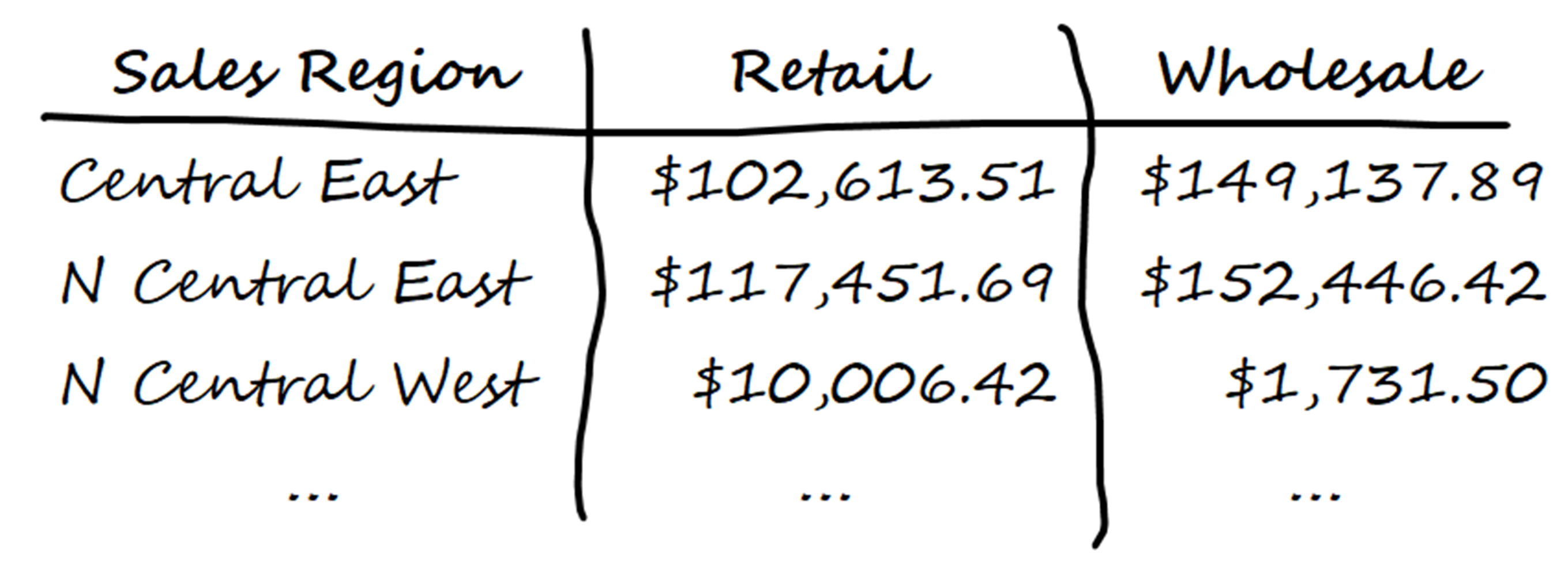
Before you create a pivot table, you should first consider how you want the data to be displayed. One approach would be to have a separate column for each product category and a separate row for each region. The total sales for each product category for each region could then be placed in the intersection of each row and column.

After thinking it through, you scribble down some thoughts and calculate some sample results to help you visualize what you want:

You’re happy with this, so next you need to translate your plan into the parameters required by the DataFrame.pivot_table() method. In this case, the parameters you need are values, index, columns, and aggfunc. It’s important to understand what these are for because they’re the core parameters used in most pivot tables.

Your pivot table will perform its calculations based on the sale price figures. These become the values passed to the values parameter, giving your pivot table the figures it needs to work with. If you don’t specify this parameter, the pivot table will use all numeric columns by default.

The index parameter is where you specify how the data is to be grouped. Remember, you need to find the total sales for each type of order for each region. You’ve decided to produce a row of aggregated data based on the sales_region field, so this will be passed as the index parameter.

You also want a separate column for each order type. This will be assigned to the columns parameter.

Finally, you also need to tell your pivot table that you want to calculate the total sales for each aggregation. To create a simple pivot table, you set its aggfunc parameter to, in this case, the sum() function.

Now that you’ve fully thought through your plan, you can go ahead and code your pivot table:

>>> pd.set_option("display.float_format", "${:,.2f}".format)

>>> sales_data.pivot_table(
...     values="sale_price", index="sales_region", columns="order_type",
...     aggfunc="sum",
... )
order_type          Retail   Wholesale
sales_region
Central East   $102,613.51 $149,137.89
N Central East $117,451.69 $152,446.42
N Central West  $10,006.42   $1,731.50
Northeast       $84,078.95 $127,423.36
Northwest       $34,565.62  $33,240.12
S Central East $130,742.32 $208,945.73
S Central West  $54,681.80  $51,051.03
Southeast       $96,310.12 $127,554.60
Southwest      $104,743.52 $121,977.20

As you can see, .pivot_table() used the parameters you planned earlier to produce your pivot table.

To format the numbers as currency, you used Python’s string format mini-language. This language is used in several places in Python, most commonly in f-strings. If you’re already familiar with it in that context, you already have the heads-up on how to use it here.

By passing "display.float_format" and "${:,.2f}".format to pandas’ set_option() function, you define the format for floating-point numbers from this point forward. They will be rounded to 2 decimal places, use a comma (,) as their thousands separator, and be prefixed with a ($) currency symbol.

Unless you want to keep this format for your future floating-point numbers, you’ll need to reset the formatting to its default by using pd.reset_option("display.float_format") after .pivot_table() has been called.

>>> with pd.option_context("display.float_format", "${:,.2f}".format):
...     sales_data.pivot_table(
...         values="sale_price", index="sales_region",
...         columns="order_type", aggfunc="sum",
...     )

While you’re basically happy with your result, you feel that something is missing: totals. You hadn’t initially thought about including totals columns, but now realize this would be useful. To fix this, you consult the documentation and come up with the following solution:

>>> pd.set_option("display.float_format", "${:,.2f}".format)

>>> sales_data.pivot_table(
...     values="sale_price", index="sales_region", columns="order_type",
...     aggfunc="sum", margins=True, margins_name="Totals",
... )
order_type          Retail   Wholesale        Totals
sales_region
Central East   $102,613.51 $149,137.89   $251,751.40
N Central East $117,451.69 $152,446.42   $269,898.11
N Central West  $10,006.42   $1,731.50    $11,737.92
Northeast       $84,078.95 $127,423.36   $211,502.31
Northwest       $34,565.62  $33,240.12    $67,805.74
S Central East $130,742.32 $208,945.73   $339,688.05
S Central West  $54,681.80  $51,051.03   $105,732.83
Southeast       $96,310.12 $127,554.60   $223,864.72
Southwest      $104,743.52 $121,977.20   $226,720.72
Totals         $735,193.95 $973,507.85 $1,708,701.80

This time, to add some additional finishing touches, you set margins=True and margins_name="Totals". The parameter margins=True added new columns onto the right and bottom of your pivot table. Each contains the totals of the rows and columns, respectively. The margins_name parameter inserted "Totals" labels instead of the default "All" labels that would appear otherwise.

Now it’s your turn. Try the following exercise to test your understanding:

If you’ve made it this far, you now understand the most important principles of creating pivot tables. Congratulations! But don’t relax just yet because there are still more exciting things for you to learn. Read on to enhance your knowledge even further.

Including Sub-Columns in Your Pivot Table

In each of your previous pivot tables, you assigned a single DataFrame Series to its columns parameter. This inserted a separate column in your pivot table for each unique entry within the assigned Series. So by assigning "order_type" to columns, your pivot table included both Retail and Wholesale columns, one for each type of order. It’s time to expand your knowledge further and learn how to include sub-columns in your pivot table.

Here’s the next milestone for you:

Calculate the average sales of the different types of orders placed by each type of customer for each state.

As before, stop and think. The first step is to think through what you want to see and fit the relevant parameters into your plan.

One way would be to display each customer’s state in a row by itself. As far as which columns to display, you could have a separate column for each type of customer and then have sub-columns for each type of order within each type of customer. The calculation will again be based on the sale price, except you need to work out their averages this time.

You get your pencil and paper out once more and create a quick visualization:

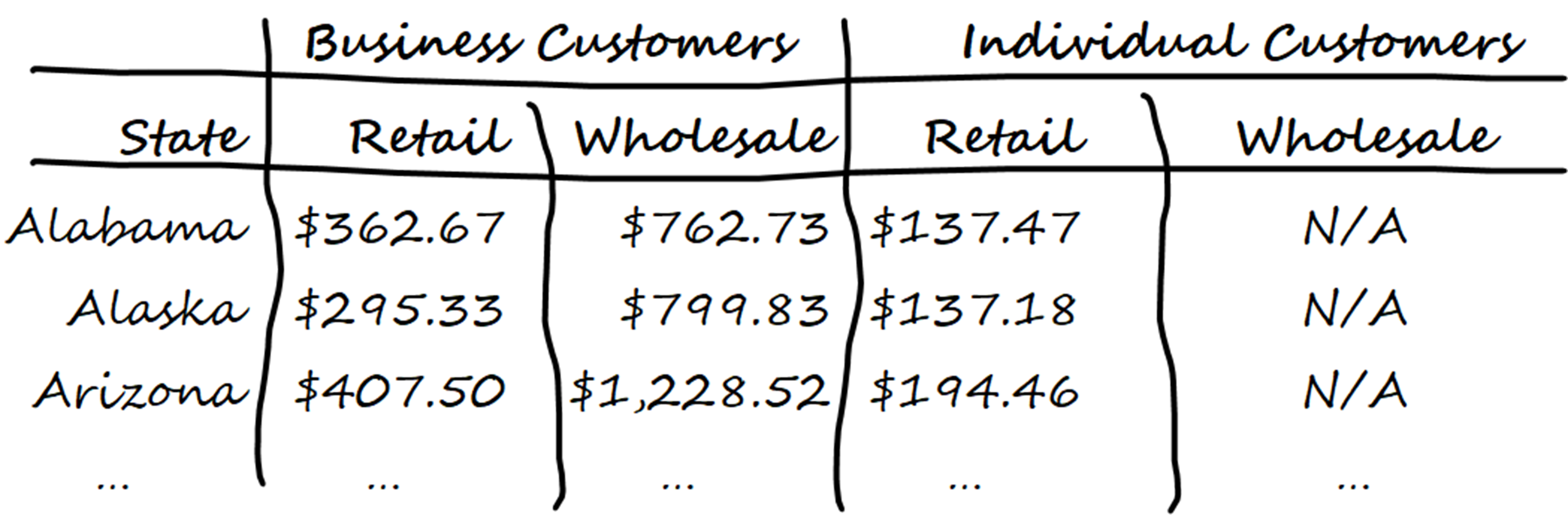
Now that you’ve thought this one through and are happy, you can apply your plan to the parameters. As before, the calculation will use the values in the sale_price column, so you’ll use this as your values parameter. Because you want the average values, you could set aggfunc="mean". However, since this is the default value, you don’t need to do this. Each row will be based on the customer’s state, so you’ll need to set index="customer_state".

Finally, you need to think about the columns. This time, because you want customer types as the top column with different order types for each of them, your columns parameter will be the list ["customer_type", "order_type"]. It’s possible to create multiple nested sub-columns by passing in a longer list, but two columns are fine here.

To meet your requirements, you use the code shown below:

>>> pd.set_option("display.float_format", "${:,.2f}".format)

>>> sales_data.pivot_table(
...     values="sale_price", index="customer_state",
...     columns=["customer_type", "order_type"], aggfunc="mean",
... )
customer_type        Business           Individual
order_type             Retail Wholesale     Retail
customer_state
Alabama               $362.67   $762.73    $137.47
Alaska                $295.33   $799.83    $137.18
Arizona               $407.50 $1,228.52    $194.46
Arkansas                 <NA> $1,251.25    $181.65
California            $110.53 $1,198.89    $170.94
...

As you can see, passing the list of columns has produced the required analysis for you. Once again, you applied an appropriate format string to keep your output readable. There were no retail sales from businesses in Arkansas, which is why it shows as <NA>. Note that the default behavior of the aggfunc parameter is to calculate the mean of the data, but you included it here only for clarity.

Now, take a look back at your original visualization and compare it to what your code actually produced. Do you notice anything different? That’s right, there’s no Individual Wholesale column in your output. This is because there are no corresponding values to put in it. The .pivot_table() method removed it automatically to prevent the display of an empty column.

It’s time for another checkpoint of your understanding. See if you can solve this next challenge:

Now that you know how to work with sub-columns, it’s time to learn how to use sub-rows.

Including Sub-Rows in Your Pivot Table

In the previous section, you saw how passing a list into the columns parameter allows you to create sub-columns. You may have already guessed that to analyze traffic by one row within another, you pass a list into the index parameter. As before, you can better understand this with an example, so here’s your next milestone:

Calculate the total sales of each of your different product categories, but also show details of the different types of orders placed by the different types of customers.

As usual, take a step back and start planning your solution carefully.

One way to solve this problem would be to have a separate column for each category of product, and a separate row analyzing the order types within the customer types. Once more, you’re going to work with totals of sales figures.

Sharpen up your pencil:

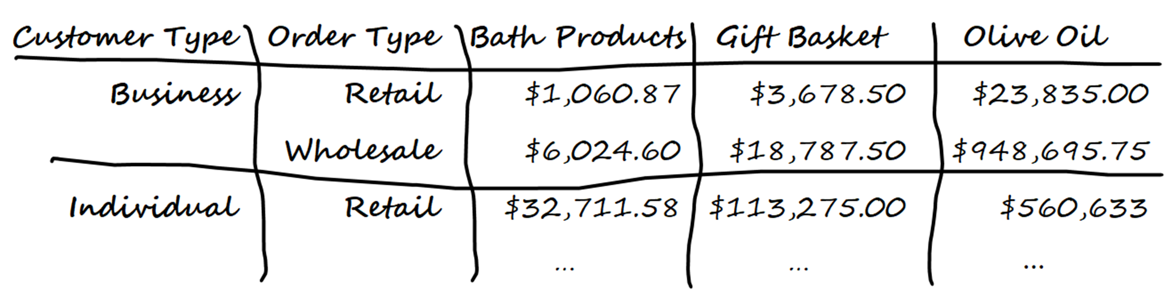
The calculation will be based on sale price, which will be your values parameter, while setting aggfunc="sum" will ensure totals are calculated. To separate each product category into its own column, you assign this to the columns parameter. Finally, to make sure the customer type is sub-analyzed by order type, you assign ["customer_type", "order_type"] to the index parameter.

When you transform your plan into code, this is the result:

>>> pd.set_option("display.float_format", "${:,.2f}".format)

>>> sales_data.pivot_table(
...     values="sale_price", index=["customer_type", "order_type"],
...     columns="product_category", aggfunc="sum",
... )
product_category          Bath products  Gift Basket   Olive Oil
customer_type order_type
Business      Retail          $1,060.87    $3,678.50  $23,835.00
              Wholesale       $6,024.60   $18,787.50 $948,695.75
Individual    Retail         $32,711.58  $113,275.00 $560,633.00
...

Here, you learned that by passing a list of columns into index, you could produce the required analysis. Once again, you used ${:,.2f} to make sure the currency was formatted correctly.

Time for your next knowledge check. See if you can solve the following:

Now that you know how to work with sub-columns and sub-rows, you might think that you’re finished. But there’s more! Next, you’ll learn how to include multiple values in your calculations.

Calculating Multiple Values in Your Pivot Table

So far, each of your pivot tables has analyzed data from a single column such as sale_price or quantity. Suppose you wanted to analyze data from both columns in the same way. Can you guess how to do it? If you’re thinking of supplying both columns in a list to the values parameter, you’re spot on.

Based on your progress so far, the next milestone is within your reach:

Calculate the sum of both the sale prices and quantities sold of each category of product within each sales region.

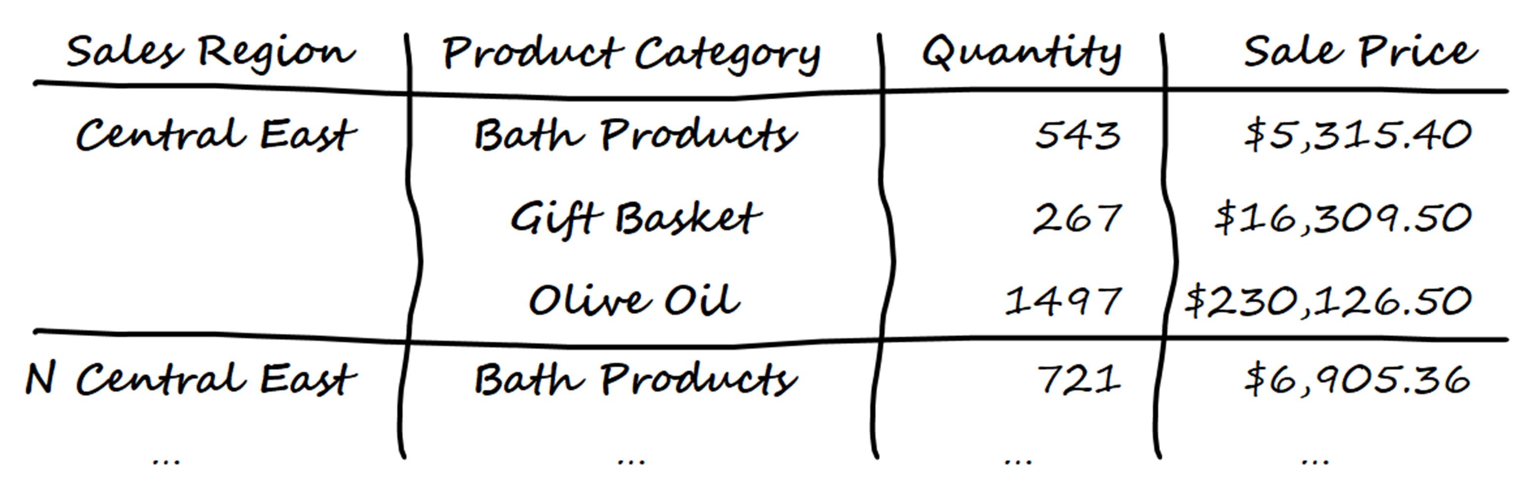
Almost subconsciously, your brain has entered planning mode:

One solution would be to produce rows for each category of product within each sales region, and then to display the total quantity and sale price for each in separate columns. In other words, you think about creating something like this:

To implement this, you use principles similar to those you used earlier, but there are one or two caveats you need to be mindful of. To calculate totals, you set aggfunc="sum", while to deal with any <NA> values by replacing them with zero, you set fill_value to 0. To produce the rows showing sales region sub-analyzed by product category, you pass them both in a list to index.

The code you could use to do all of this is shown below:

>>> pd.set_option("display.float_format", "${:,.2f}".format)

>>> sales_data.pivot_table(
...     index=["sales_region", "product_category"],
...     values=["sale_price", "quantity"],
...     aggfunc="sum", fill_value=0,
... )
                                 quantity  sale_price
sales_region   product_category
Central East   Bath Products          543   $5,315.40
               Gift Basket            267  $16,309.50
               Olive Oil             1497 $230,126.50
N Central East Bath Products          721   $6,905.36
               Gift Basket            362  $21,533.00
               Olive Oil             1648 $241,459.75
N Central West Bath Products           63     $690.92
               Gift Basket             26   $2,023.50
               Olive Oil               87   $9,023.50
...

To calculate the totals of both sale_price and quantity, you passed them in as a list to the values parameter. One small issue is that the calculation columns are displayed differently from the order of their defining list. In this example, you passed in ["sale_price", "quantity"] to values, but if you look carefully at the output, you’ll see it’s displayed alphabetically.

Once again, you used "${:,.2f}" to make sure the currency was formatted correctly. Note that this only applies to floats. The formatting of the quantity integer values took care of themselves.

One other point to note is that there’s no columns parameter. You may have thought that the list passed to values should have been passed to columns, but this is not the case. The columns parameter, as well as index, allow you to define how data is grouped. In this example, you’re not grouping by sale price or quantity. Instead, you’re using them in a calculation. Therefore, they must be assigned to values.

>>> pd.set_option("display.float_format", "${:,.2f}".format)

>>> sales_data.pivot_table(
...     index=["sales_region", "product_category"],
...     values=["sale_price", "quantity"],
...     aggfunc="sum", fill_value=0,
... ).loc[:, ["sale_price", "quantity"]]

It’s time to massage that gray matter once more. See if you can solve the next challenge:

By now, you’re turning into a competent creator of pivot tables. You may wonder what else there’s left to learn. If you want to know how to apply different aggregation functions to the same data, different aggregation functions to different data, or even how to write your own custom aggregation functions, read on.

Performing More Advanced Aggregations

Now that you’re flying high with confidence, you wonder if you can do the following:

Calculate the maximum and minimum sales of each category of product for each type of customer.

With your brain’s cooling system now on full power, you can start to think things through once more.

To solve this, you need to apply multiple aggregation functions to the same data. Previously, when you analyzed data using multiple criteria, you did so by passing lists to an appropriate parameter. Can you guess how to apply multiple functions? If not, the answer is shown below:

>>> pd.set_option("display.float_format", "${:,.2f}".format)

>>> sales_data.pivot_table(
...     values=["sale_price"], index="product_category",
...     columns="customer_type", aggfunc=["max", "min"],
... )
                        max                   min
                 sale_price            sale_price
customer_type      Business Individual   Business Individual
product_category
Bath Products       $300.00    $120.00      $5.99      $5.99
Gift Basket       $1,150.00    $460.00     $27.00     $19.50
Olive Oil         $3,276.00    $936.00     $16.75     $16.75

Here you applied multiple functions to the same data by passing them in as a list to the aggfunc parameter. You also decided to create a row for each product category, and this became the index parameter. Your calculations were based on sale price, so you passed that as the values parameter. Since you passed it in as a list, you ensured that the heading sale price appears as an additional column heading for clearer readability.

Also, because you wanted to see data by customer type, you decided to make this the columns parameter. To perform both a "max" and "min" calculation, you passed in both of these to the aggfunc parameter within a list.

Next, you decide to push the boat out a little further as you try this:

Adjust the previous analysis to display both the average sale price and the maximum quantity sold.

Thinking it through, you realize that this would be an example of applying different aggregation functions to different data. To do this, you need to pass not a list, but a dictionary to aggfunc that defines each data column and aggregation function to be used on it. Don’t forget to make sure each piece of data appears in the values parameter as well.

To create this pivot table, you could do the following:

>>> pd.set_option("display.float_format", "${:,.2f}".format)

>>> sales_data.pivot_table(
...     values=["sale_price", "quantity"],
...     index=["product_category"],
...     columns="customer_type",
...     aggfunc={"sale_price": "mean", "quantity": "max"},
... )
                 quantity            sale_price
customer_type    Business Individual   Business Individual
product_category
Bath Products          14          4     $53.27     $25.94
Gift Basket            14          4    $335.31    $156.24
Olive Oil              14          4  $1,385.37    $250.06

The pivot table now shows the maximum quantities for each of the two customer types and the average sale price for each. You achieved this by appending quantity to the values parameter’s list, and then you passed a dictionary into aggfunc before .pivot_table() worked its magic.

You move on and shove that boat out even further still as you do this:

Calculate how many employees there are in each sales region.

At first glance, this appears simple. You quickly think it through and believe this code will give you what you want:

>>> sales_data.pivot_table(
...     values="employee_id",
...     index="sales_region",
...     aggfunc="count",
... )
                employee_id
sales_region
Central East            697
N Central East          832
N Central West           70
Northeast               604
...

When you run this code, there appears to be plenty of salespeople in each region. These figures are incorrect because count has counted duplicate employee_id values. If you take a look back at the original data, you’ll see that the same employee is listed multiple times within their sales region. You need to have a re-think.

Up to this point, you’ve used the aggfunc parameter to specify the functions used to perform the aggregation calculations. Each of these took the series defined by the values parameter and aggregated it into a single value according to the index and columns parameters. You can take these ideas a step further and write your own custom aggregation function, provided it takes a series as its argument and returns a single aggregated value.

As you write your own aggregation function, you need to pass in a sub-series of employee_id values for each sales_region. Your function then needs to work out how many unique values are in each sub-series and return the results back to .pivot_table(). One way to write such a function is shown below:

>>> def count_unique(values):
...     return len(values.unique())
...

Your count_unique() function accepted a pandas Series named values and used the Series.unique() method to obtain a NumPy array containing the unique elements of the Series. The Python built-in len() function then returned the length, or number of elements, in each values Series.

To call your function and pass the various sub-series to it, you assign the function’s name to the aggfunc parameter of .pivot_table(). Fortunately, you don’t need to worry about passing each sub-series because this is done for you by .pivot_table(). This means your function is called once for each different sales region. The return values are then displayed in the resulting pivot table.

To see how this works, take a look at the code below:

>>> sales_data.pivot_table(
...     values="employee_id",
...     index=["sales_region"],
...     aggfunc=count_unique,
... )
                employee_id
sales_region
Central East              6
N Central East            6
N Central West            1
Northeast                 4
...

As you can see, by assigning count_unique to the aggfunc parameter, .pivot_table() calculated the number of unique employee id values. In other words, it calculated the number of sales staff there are in each region. Yet another success!

Time for another challenge. Have fun with this one:

At this stage, you’ve now become an expert at creating pivot tables in Python. Finally, you’ll learn about other ways to aggregate data.

Using .groupby() and crosstab() for Aggregation

Although your pivot table experience so far has been focused on .pivot_table(), this is not the only way to perform data aggregation in pandas. DataFrames also has a .groupby() method, while pandas provides a crosstab() function that also aggregates data. In this section, you’ll see examples of how they can be used to do more than .pivot_table().

One feature you might find useful that exists within .groupby() but not .pivot_table() is named aggregations. These allow you to apply custom column headings to clarify the display of your aggregated calculations.

Here’s your next learning milestone:

Calculate the lowest, average, highest, and standard deviation of the prices of each product category, then use named aggregations to improve your output.

You decide to use your existing knowledge to plan and write the following code. You’re confident this will at least let you see the data figures you need:

>>> sales_data.pivot_table(
...     values="sale_price",
...     index="product_category",
...     aggfunc=["min", "mean", "max", "std"],
... )
                        min       mean        max        std
                 sale_price sale_price sale_price sale_price
product_category
Bath Products         $5.99     $28.55    $300.00     $23.98
Gift Basket          $19.50    $171.39  $1,150.00    $131.64
Olive Oil            $16.75    $520.78  $3,276.00    $721.49

The above code analyzed your data by product category and calculated the minimum, average, maximum, and standard deviation of the sale price. However, while this output certainly gave you what you wanted, the column headings showing each sale price are not very well presented. This is where named aggregations can help.

To perform an aggregation calculation using .groupby(), you pass it the column or columns you want to group by. This returns something called a DataFrameGroupBy object, which contains an .agg() method that allows you to define the aggregation functions to be used, as well as their headings.

One way you can use .agg() is to pass it one or more tuples containing the data column and aggregation function to be used for that column. You pass each tuple in using a keyword, which becomes the name of the heading in the resulting aggregation.

The above example could be written with .groupby() as shown below:

>>> (
...     sales_data
...     .groupby("product_category")
...     .agg(
...          low_price=("sale_price", "min"),
...          average_price=("sale_price", "mean"),
...          high_price=("sale_price", "max"),
...          standard_deviation=("sale_price", "std"),
...     )
... )
                  low_price  average_price  high_price  standard_deviation
product_category
Bath Products         $5.99         $28.55     $300.00              $23.98
Gift Basket          $19.50        $171.39   $1,150.00             $131.64
Olive Oil            $16.75        $520.78   $3,276.00             $721.49

This time, you can see that the data is once more grouped by product category, but each grouping has a neater heading named after the keyword used to specify the tuple. If you’re interested in diving deeper into .groupby() and how to use it, check out pandas GroupBy: Your Guide to Grouping Data in Python.

One other common way to create an aggregation is to use the crosstab() function. This has similar functionality to .pivot_table() because, as you learned earlier, it uses .pivot_table() to perform its analysis. The major difference is that data is passed to crosstab() as an individual pandas Series.

Your final milestone is:

Calculate the count of the staff in each region analyzed by job title using crosstab().

As you read through the documentation, you soon realize that the parameters of crosstab() are similar to those of pivot_table(). This means you know more about crosstab() than you first thought. Your existing knowledge allows you to quickly plan and run the following code:

>>> pd.crosstab(
...     index=sales_data["job_title"],
...     columns=sales_data["sales_region"],
...     margins=True,
...     margins_name="Totals",
... )
sales_region                 Central East  N Central East \
job_title
Sales Associate                         0             132
Sales Associate I                       0               0
Sales Associate II                    139               0
Sales Associate III                     0               0
...
Totals                                697             832

N Central West  ...  Southeast  Southwest  Totals
                ...
             0  ...          0        138      357
            70  ...        195        254      929
             0  ...          0         95      727
             0  ...        231          0      358
                ...
            70  ...        694        731     5130
[10 rows x 10 columns]

The parameters used by crosstab() are similar to those used by pivot_table(). Indeed, in the example above, each parameter has the same effect as its pivot_table() equivalent. The only difference is that the crosstab() function must have its data series passed in using a DataFrame reference, meaning data can be sourced from multiple DataFrames. In this example, each row is analyzed by job title, while each column is analyzed by sales region.

One feature supported by crosstab() that’s not included in .pivot_table() is the normalize parameter. When you set normalize=True, you divide each cell by the total of all the other cells in the resulting DataFrame:

>>> pd.set_option("display.float_format", "{:.2%}".format)

>>> pd.crosstab(
...     index=sales_data["job_title"],
...     columns=sales_data["sales_region"],
...     margins=True,
...     margins_name="Totals",
...     normalize=True,
... )
sales_region                Central East N Central East \
job_title
Sales Associate                    0.00%          2.57%
Sales Associate I                  0.00%          0.00%
Sales Associate II                 2.71%          0.00%
Sales Associate III                0.00%          0.00%
...
Totals                            13.59%         16.22%

N Central West  ... Southeast Southwest  Totals
                ...
         0.00%  ...     0.00%     2.69%    6.96%
         1.36%  ...     3.80%     4.95%   18.11%
         0.00%  ...     0.00%     1.85%   14.17%
         0.00%  ...     4.50%     0.00%    6.98%
                ...
         1.36%  ...    13.53%    14.25%  100.00%

[10 rows x 10 columns]

This code is very similar to the previous example, except that by setting normalize=True, you calculated each figure as a percentage of the total. You also used "{:.2%}" to display the output in conventional percentage format.

Conclusion

You now have a comprehensive understanding of how to use the .pivot_table() method, its core parameters, and how they’re used to structure pivot tables. Most importantly, you learned the importance of thinking through what you want to achieve before implementing it.

You also learned how to create a pivot table using the DataFrame.pivot_table() method’s main parameters and how some parameters can produce a more detailed analysis with lists of values instead of single values. To round off your knowledge of .pivot_table(), you learned how to create pivot tables that perform multiple aggregations, column-specific aggregations, and even custom aggregations.

You were also introduced to two other ways of aggregating data using .groupby() and crosstab(), which you can continue to investigate on your own to expand your knowledge even further. Now, you can confidently produce interesting and complex views of data to allow the insights within it to be revealed.

Congratulations on completing this tutorial, and enjoy applying these newfound skills to your future data analysis projects!

Take the Quiz: Test your knowledge with our interactive “How to Create Pivot Tables With pandas” quiz. You’ll receive a score upon completion to help you track your learning progress:

---

Interactive Quiz

How to Create Pivot Tables With pandas

This quiz is designed to push your knowledge of pivot tables a little bit further. You won't find all the answers by reading the tutorial, so you'll need to do some investigating on your own. By finding all the answers, you're sure to learn some other interesting things along the way.