This tutorial will guide you through a fun project involving complex numbers in Python. You’re going to learn about fractals and create some truly stunning art by drawing the Mandelbrot set using Python’s Matplotlib and Pillow libraries. Along the way, you’ll learn how this famous fractal was discovered, what it represents, and how it relates to other fractals.
Knowing about object-oriented programming principles and recursion will enable you to take full advantage of Python’s expressive syntax to write clean code that reads almost like math formulas. To understand the algorithmic details of making fractals, you should also be comfortable with complex numbers, logarithms, set theory, and iterated functions. But don’t let these prerequisites scare you away, as you’ll be able to follow along and produce the art anyway!
In this tutorial, you’ll learn how to:
- Apply complex numbers to a practical problem
- Find members of the Mandelbrot and Julia sets
- Draw these sets as fractals using Matplotlib and Pillow
- Make a colorful artistic representation of the fractals
To download the source code used in this tutorial, click the link below:
Get Source Code: Click here to get the source code you’ll use to draw the Mandelbrot set.
Understanding the Mandelbrot Set
Before you try to draw the fractal, it’ll help to understand what the corresponding Mandelbrot set represents and how to determine its members. If you’re already familiar with the underlying theory, then feel free to skip ahead to the plotting section below.
The Icon of Fractal Geometry
Even if the name is new to you, you might have seen some mesmerizing visualizations of the Mandelbrot set before. It’s a set of complex numbers, whose boundary forms a distinctive and intricate pattern when depicted on the complex plane. That pattern became arguably the most famous fractal, giving birth to fractal geometry in the late 20th century:

The discovery of the Mandelbrot set was possible thanks to technological advancement. It’s attributed to a mathematician named Benoît Mandelbrot. He worked at IBM and had access to a computer capable of what was, at the time, demanding number crunching. Today, you can explore fractals in the comfort of your home, using nothing more than Python!
Fractals are infinitely repeating patterns on different scales. While philosophers have argued for centuries about the existence of infinity, fractals do have an analogy in the real world. It’s a fairly common phenomenon occurring in nature. For example, this Romanesco cauliflower is finite but has a self-similar structure because each part of the vegetable looks like the whole, only smaller:

Self-similarity can often be defined mathematically with recursion. The Mandelbrot set isn’t perfectly self-similar as it contains slightly different copies of itself at smaller scales. Nevertheless, it can still be described by a recursive function in the complex domain.
The Boundary of Iterative Stability
Formally, the Mandelbrot set is the set of complex numbers, c, for which an infinite sequence of numbers, z0, z1, …, zn, …, remains bounded. In other words, there is a limit that the magnitude of each complex number in that sequence never exceeds. The Mandelbrot sequence is given by the following recursive formula:

In plain English, to decide whether some complex number, c, belongs to the Mandelbrot set, you must feed that number to the formula above. From now on, the number c will remain constant as you iterate the sequence. The first element of the sequence, z0, is always equal to zero. To calculate the next element, zn+1, you’ll keep squaring the last element, zn, and adding your initial number, c, in a feedback loop.
By observing how the resulting sequence of numbers behaves, you’ll be able to classify your complex number, c, as either a Mandelbrot set member or not. The sequence is infinite, but you must stop calculating its elements at some point. Making that choice is somewhat arbitrary and depends on your accepted level of confidence, as more elements will provide a more accurate ruling on c.
Note: The entire Mandelbrot set fits in a circle with a radius of two when depicted on the complex plane. This is a handy fact that’ll let you skip many unnecessary calculations for points that certainly don’t belong to the set.
With complex numbers, you can imagine this iterative process visually in two dimensions, but you can go ahead and consider only real numbers for the sake of simplicity now. If you were to implement the above equation in Python, then it could look something like this:
>>> def z(n, c):
...     if n == 0:
...         return 0
...     else:
...         return z(n - 1, c) ** 2 + c
Your z() function returns the nth element of the sequence, which is why it expects an element’s index, n, as the first argument. The second argument, c, is a fixed number that you’re testing. This function would keep calling itself infinitely due to recursion. However, to break that chain of recursive calls, a condition checks for the base case with an immediately known solution—zero.
Try using your new function to find the first ten elements of the sequence for c = 1, and see what happens:
>>> for n in range(10):
...     print(f"z({n}) = {z(n, c=1)}")
...
z(0) = 0
z(1) = 1
z(2) = 2
z(3) = 5
z(4) = 26
z(5) = 677
z(6) = 458330
z(7) = 210066388901
z(8) = 44127887745906175987802
z(9) = 1947270476915296449559703445493848930452791205
Notice the rapid growth rate of these sequence elements. It tells you something about the membership of c = 1. Specifically, it does not belong to the Mandelbrot set, because the corresponding sequence grows without bound.
Sometimes, an iterative approach might be more efficient than a recursive one. Here’s an equivalent function that creates an infinite sequence for the specified input value, c:
>>> def sequence(c):
...     z = 0
...     while True:
...         yield z
...         z = z ** 2 + c
The sequence() function returns a generator object yielding consecutive elements of the sequence endlessly in a loop. Because it doesn’t return the corresponding element indices, you can enumerate them and stop the loop after a given number of iterations:
>>> for n, z in enumerate(sequence(c=1)):
...     print(f"z({n}) = {z}")
...     if n >= 9:
...         break
...
z(0) = 0
z(1) = 1
z(2) = 2
z(3) = 5
z(4) = 26
z(5) = 677
z(6) = 458330
z(7) = 210066388901
z(8) = 44127887745906175987802
z(9) = 1947270476915296449559703445493848930452791205
The result is the same as before, but the generator function lets you calculate the sequence elements more efficiently by using lazy evaluation. In addition to this, iteration eliminates redundant function calls for the already-computed sequence elements. As a consequence, you’re not running the risk of hitting the maximum recursion limit anymore.
Most numbers will make this sequence diverge to infinity. However, some will keep it stable by either converging the sequence to a single value or staying within a bounded range. Others will make the sequence periodically stable by cycling back and forth between the same few values. Stable and periodically stable values make up the Mandelbrot set.
For example, plugging in c = 1 makes the sequence grow without bound like you just learned, but c = -1 causes it to jump between 0 and -1 repeatedly, while c = 0 gives a sequence comprised of a single value:
| Element | c = -1 | c = 0 | c = 1 |
|---|---|---|---|
| z0 | 0 | 0 | 0 |
| z1 | -1 | 0 | 1 |
| z2 | 0 | 0 | 2 |
| z3 | -1 | 0 | 5 |
| z4 | 0 | 0 | 26 |
| z5 | -1 | 0 | 677 |
| z6 | 0 | 0 | 458,330 |
| z7 | -1 | 0 | 210,066,388,901 |
It’s not obvious which numbers are stable and which aren’t, because the formula is sensitive to even the smallest change of the tested value, c. If you mark the stable numbers on the complex plane, then you’ll see the following pattern emerge:
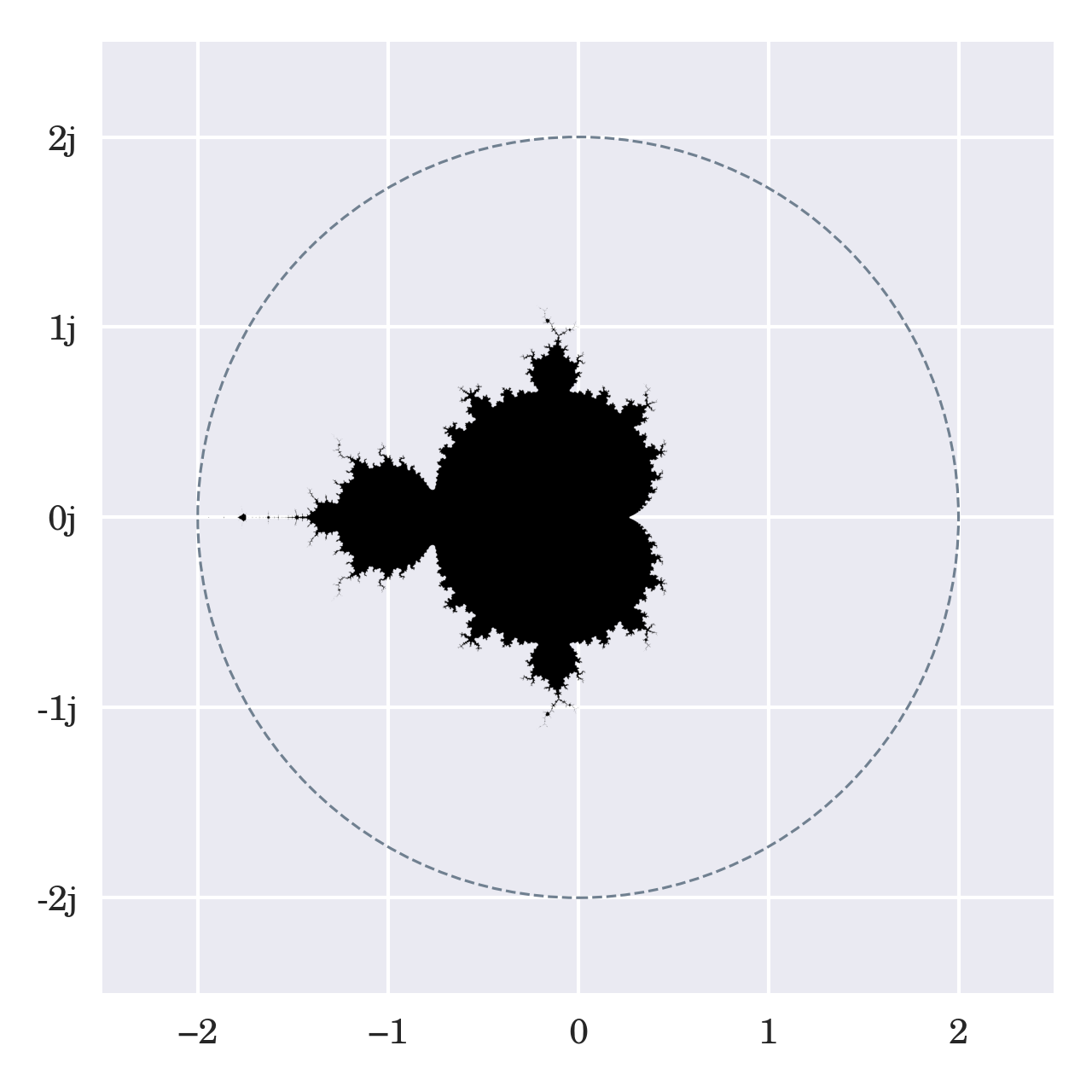
This image has been generated by running the recursive formula up to twenty times per pixel, with each pixel representing some c value. When the magnitude of the resulting complex number was still reasonably small after all iterations, then the corresponding pixel was colored black. However, as soon as the magnitude exceeded the radius of two, then the iteration stopped and skipped the current pixel.
Fun Fact: The fractal corresponding to the Mandelbrot set has a finite area estimated at 1.506484 square units. Mathematicians haven’t pinpointed the exact number yet and don’t know whether it’s rational or not. On the other hand, the perimeter of the Mandelbrot set is infinite. Check out the coastline paradox to learn about an interesting parallel of this weird fact in real life.
You may find it astonishing that a relatively simple formula that only involves addition and multiplication can produce such an elaborate structure. But that’s not all. It turns out that you can take the same formula and use it to generate infinitely many unique fractals! Do you want to see how?
The Map of Julia Sets
It’s hard to talk about the Mandelbrot set without mentioning Julia sets, which had been discovered by French mathematician Gaston Julia several decades earlier without the help of computers. Julia sets and the Mandelbrot set are closely related because you can obtain them through the same recursive formula, only with different sets of starting conditions.
While there’s only one Mandelbrot set, there are infinitely many Julia sets. So far, you always started the sequence at z0 = 0 and systematically tested some arbitrary complex number, c, for its membership. On the other hand, to find out if a number belongs to a Julia set, you must use that number as the starting point for the sequence and pick another value for the c parameter.
Here’s a quick comparison of the formula’s terms depending on which set you’re investigating:
| Term | Mandelbrot Set | Julia Set |
|---|---|---|
| z0 | 0 | Candidate value |
| c | Candidate value | Fixed constant |
In the first case, c represents a potential member of the Mandelbrot set and is the only input value required because z0 remains fixed at zero. However, each term changes its meaning when you use the formula in Julia mode. Now, c works as a parameter that determines the shape and form of an entire Julia set, while z0 becomes your point of interest. Unlike before, the formula for a Julia set expects not one but two input values.
You can modify one of your functions defined before to make it more generic. This way, you can create infinite sequences starting at any point rather than always zero:
def sequence(c, z=0):
    while True:
        yield z
        z = z ** 2 + c
Thanks to the default argument value in the highlighted line, you can still use this function as before because z is optional. At the same time, you may change the starting point of the sequence. Perhaps you’ll get a better idea after defining wrapper functions for the Mandelbrot and Julia sets:
def mandelbrot(candidate):
    return sequence(z=0, c=candidate)

def julia(candidate, parameter):
    return sequence(z=candidate, c=parameter)
Each function returns a generator object fine-tuned to your desired starting condition. The principles for determining whether a candidate value belongs to a Julia set are similar to the Mandelbrot set that you saw earlier. In a nutshell, you must iterate the sequence and observe its behavior over time.
Benoît Mandelbrot was, in fact, studying Julia sets in his scientific research. He was particularly interested in finding those values of c that produce so-called connected Julia sets as opposed to their disconnected counterparts. The latter are known as Fatou sets and appear as dust comprised of an infinite number of pieces when visualized on the complex plane:
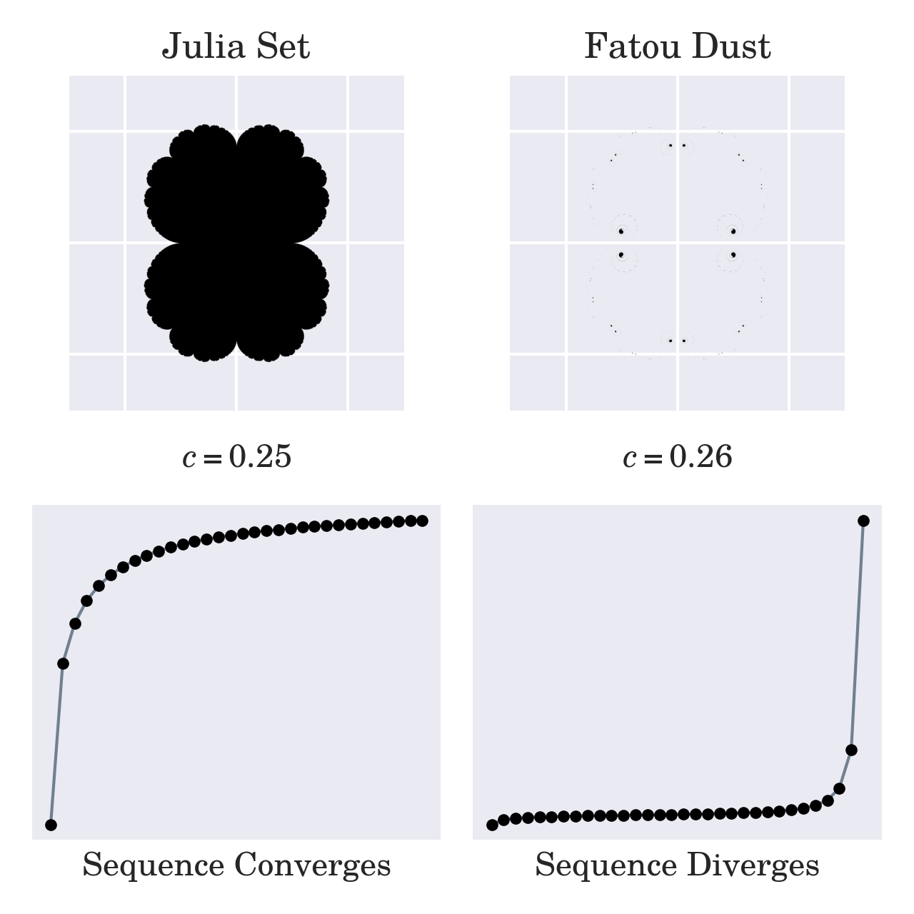
The image in the top-left corner represents a connected Julia set derived from c = 0.25, which belongs to the Mandelbrot set. You know that plugging a member of the Mandelbrot set into the recursive formula will produce a sequence of complex numbers that converge. The numbers converge to 0.5 in this case. However, a slight change to c can suddenly turn your Julia set into disconnected dust and make the corresponding sequence diverge to infinity.
Coincidentally, the connected Julia sets correspond to c values that generate stable sequences of the recursive formula above. So, you might say that Benoît Mandelbrot was looking for the boundary of iterative stability, or a map of all the Julia sets that would show where those sets are connected and where they are dust.
Watch how choosing different points for the c parameter on the complex plane affects the resulting Julia set:
The little moving red circle indicates the value of c. As long as it stays inside the Mandelbrot set shown on the left-hand side, the corresponding Julia set depicted to the right remains connected. Otherwise, the Julia set pops like a bubble spreading into infinitely many dusty pieces.
Did you notice how the Julia sets are changing shape? It turns out that a particular Julia set shares common visual features with the specific area of the Mandelbrot set used to seed the value of c. When you look through a magnifying glass, then both fractals will appear somewhat similar.
Okay, enough theory. Time to plot your first Mandelbrot set!
Plotting the Mandelbrot Set Using Python’s Matplotlib
There are plenty of ways to visualize the Mandelbrot set in Python. If you’re comfortable with NumPy and Matplotlib, then these two libraries together will provide one of the most straightforward ways to plot the fractal. They conveniently spare you from having to convert between the world and pixel coordinates.
Note: World coordinates correspond to the continuous spectrum of numbers on the complex plane, extending to infinity. On the other hand, pixel coordinates are discrete and constrained by the finite size of your screen.
To generate the initial set of candidate values, you can take advantage of np.linspace(), which creates evenly spaced numbers in a given range:
 1import numpy as np
 2
 3def complex_matrix(xmin, xmax, ymin, ymax, pixel_density):
 4    re = np.linspace(xmin, xmax, int((xmax - xmin) * pixel_density))
 5    im = np.linspace(ymin, ymax, int((ymax - ymin) * pixel_density))
 6    return re[np.newaxis, :] + im[:, np.newaxis] * 1j
The function above will return a two-dimensional array of complex numbers enclosed in a rectangular area given by four parameters. The xmin and xmax parameters specify the bounds in the horizontal direction, while ymin and ymax do so in the vertical direction. The fifth parameter, pixel_density, determines the desired number of pixels per unit.
Now, you can take that matrix of complex numbers and run it through the well-known recursive formula to see which numbers remain stable and which don’t. Thanks to NumPy’s vectorization, you can pass the matrix as a single parameter, c, and perform the calculations on each element without having to write explicit loops:
 8def is_stable(c, num_iterations):
 9    z = 0
10    for _ in range(num_iterations):
11        z = z ** 2 + c
12    return abs(z) <= 2
The code on the highlighted line gets executed for all elements of matrix c on each iteration. Because z and c start with different dimensions initially, NumPy uses broadcasting to cleverly extend the former so that both end up having compatible shapes. Finally, the function creates a two-dimensional mask of Boolean values over the resulting matrix, z. Each value corresponds to the sequence’s stability at that point.
Note: To take advantage of vectorized computation, the loop in the code example keeps squaring and adding numbers unconditionally, regardless of how big they already were. That’s not ideal because, in many cases, the numbers diverge to infinity early on, making most of the computations wasteful.
Moreover, the numbers that grow quickly often lead to an overflow error. NumPy detects such overflows and issues a warning on the standard error stream (stderr). If you’d like to suppress such warnings, then you can define a relevant filter before calling your function:
 1import numpy as np
 2
 3np.warnings.filterwarnings("ignore")
Ignoring these overflows is harmless because you’re not interested in specific magnitudes but rather if they fit the given threshold.
After a chosen number of iterations, the magnitude of each complex number in the matrix will either stay within or exceed the threshold of two. Those that are small enough are likely members of the Mandelbrot set. You can now visualize them using Matplotlib.
Low-Resolution Scatter Plot
A quick and dirty way to visualize the Mandelbrot set is through a scatter plot, which illustrates the relationships between paired variables. Because complex numbers are pairs of the real and imaginary components, you can untangle them into separate arrays that’ll play nicely with the scatter plot.
But first, you need to turn your Boolean mask of stability into the initial complex numbers that seeded the sequence. You can do so with the help of NumPy’s masked filtering:
16def get_members(c, num_iterations):
17    mask = is_stable(c, num_iterations)
18    return c[mask]
This function will return a one-dimensional array comprised of only those complex numbers that are stable and therefore belong to the Mandelbrot set. When you combine the functions defined so far, you’ll be able to show a scatter plot using Matplotlib. Don’t forget to add the necessary import statement at the beginning of your file:
 1import matplotlib.pyplot as plt
 2import numpy as np
 3
 4np.warnings.filterwarnings("ignore")
This brings the plotting interface to your current namespace. Now you can calculate your data and plot it:
21c = complex_matrix(-2, 0.5, -1.5, 1.5, pixel_density=21)
22members = get_members(c, num_iterations=20)
23
24plt.scatter(members.real, members.imag, color="black", marker=",", s=1)
25plt.gca().set_aspect("equal")
26plt.axis("off")
27plt.tight_layout()
28plt.show()
The call to complex_matrix() prepares a rectangular array of complex numbers in the range of -2 to 0.5 in the x-direction and between -1.5 and 1.5 in the y-direction. The subsequent call to get_members() passes through only those numbers that are members of the Mandelbrot set. Finally, plt.scatter() plots the set, and plt.show() reveals this picture:

It contains 749 points and resembles the original ASCII printout made on a dot matrix printer by Benoît Mandelbrot himself a few decades ago. You’re reliving mathematical history! Play around by adjusting the pixel density and the number of iterations to see how they affect the outcome.
High-Resolution Black-and-White Visualization
To get a more detailed visualization of the Mandelbrot set in black and white, you can keep increasing the pixel density of your scatter plot until the individual dots become hardly discernable. Alternatively, you can use Matplotlib’s plt.imshow() function with a binary colormap to plot your Boolean mask of stability.
There are only a few tweaks necessary in your existing code:
21c = complex_matrix(-2, 0.5, -1.5, 1.5, pixel_density=512)
22plt.imshow(is_stable(c, num_iterations=20), cmap="binary")
23plt.gca().set_aspect("equal")
24plt.axis("off")
25plt.tight_layout()
26plt.show()
Bump up your pixel density to a sufficiently large value, such as 512. Then, remove the call to get_members(), and replace the scatter plot with plt.imshow() to display the data as an image. If everything goes well, then you should see this picture of the Mandelbrot set:
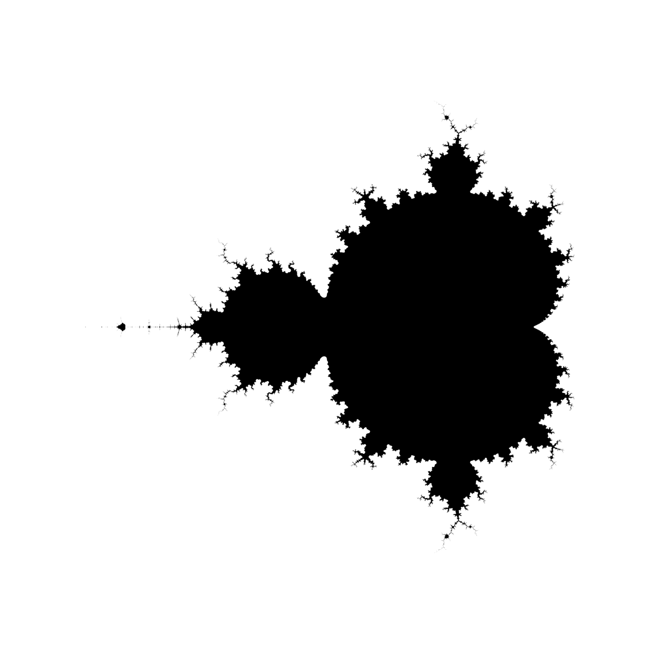
To zoom in on a particular area of the fractal, change the bounds of the complex matrix accordingly and increase the number of iterations by a factor of ten or more. You can also experiment with different colormaps provided by Matplotlib. However, to truly unleash your inner artist, you might want to get your feet wet with Pillow, Python’s most popular imaging library.
Drawing the Mandelbrot Set With Pillow
This section will require a bit more effort because you’re going to do some of the work that NumPy and Matplotlib did for you before. But having more granular control over the visualization process will let you depict the Mandelbrot set in much more interesting ways. Along the way, you’ll learn a few helpful concepts and follow the best Pythonic practices.
NumPy works with Pillow just as well as it does with Matplotlib. You can convert a Pillow image into a NumPy array with np.asarray() or the other way around using Image.fromarray(). Thanks to this compatibility, you may update your plotting code from the previous section by replacing Matplotlib’s plt.imshow() with a very similar call to Pillow’s factory method:
21c = complex_matrix(-2, 0.5, -1.5, 1.5, pixel_density=512)
22image = Image.fromarray(~is_stable(c, num_iterations=20))
23image.show()
Notice the use of the bitwise not operator (~) in front of your stability matrix, which inverts all of the Boolean values. This is so that the Mandelbrot set appears in black on a white background since Pillow assumes a black background by default.
If NumPy is your preferred tool that you’re familiar with, then feel free to incorporate it throughout this section. It’ll perform much more quickly than the pure Python code that you’re about to see because NumPy is highly optimized and relies on compiled machine code. Nevertheless, implementing the drawing code from scratch will give you the ultimate control and a deep understanding of the individual steps involved.
Fun Fact: The Pillow imaging library comes with a convenience function that can generate an image of the Mandelbrot set in one line of Python code:
from PIL import Image
Image.effect_mandelbrot((512, 512), (-3, -2.5, 2, 2.5), 100).show()
The first argument passed to the function is a tuple containing the width and height of the resulting image in pixels. The next argument defines the bounding box as bottom-left and top-right corners. The third argument is the image quality on a scale from 0 to 100.
Have a look at the corresponding C source code on GitHub if you’re interested in how the function works.
In the rest of this section, you’re going to do the hard work yourself without taking any shortcuts.
Finding Convergent Elements of the Set
Earlier, you built a stability matrix using NumPy’s vectorization to determine which of the given complex numbers belong to the Mandelbrot set. Your function iterated over the formula a fixed number of times and returned a two-dimensional array of Boolean values. Using pure Python, you can modify this function so that it works on the individual numbers rather than a whole matrix:
>>> def is_stable(c, max_iterations):
...     z = 0
...     for _ in range(max_iterations):
...         z = z ** 2 + c
...         if abs(z) > 2:
...             return False
...     return True
It looks pretty similar to NumPy’s version from before. However, there are a few important differences. Notably, the c parameter represents a single complex number, and the function returns a scalar Boolean value. Secondly, there’s an if-condition in the loop’s body, which can terminate the iteration prematurely as soon as the magnitude of the resulting number reaches a known threshold.
Note: One of the function parameters was renamed from num_iterations to max_iterations to reflect the fact that the number of iterations is no longer fixed and can vary between tested values.
You can use your new function to determine if a complex number creates a stable sequence that converges or not. That translates directly to Mandelbrot set membership. However, the result may depend on the maximum number of iterations requested:
>>> is_stable(0.26, max_iterations=20)
True
>>> is_stable(0.26, max_iterations=30)
False
For example, the number c = 0.26 is located close to the fractal’s edge, so you’ll get a wrong answer with too few iterations. Increasing the maximum number of iterations can be more accurate, revealing more details on the visualization.
There’s nothing wrong with calling a function, but wouldn’t it be nicer to leverage Python’s in and not in operators instead? Turning this code into a Python class will let you override those operators and take advantage of a much cleaner and more Pythonic syntax. Moreover, you’ll be able to retain the maximum number of iterations across many function invocations by encapsulating the state in your object.
You can take advantage of data classes to avoid having to define a custom constructor function. Here’s an equivalent class-based implementation of the same code:
# mandelbrot.py

from dataclasses import dataclass

@dataclass
class MandelbrotSet:
    max_iterations: int

    def __contains__(self, c: complex) -> bool:
        z = 0
        for _ in range(self.max_iterations):
            z = z ** 2 + c
            if abs(z) > 2:
                return False
        return True
Apart from implementing the special method .__contains__(), adding a few type hints, and moving the max_iterations parameter out from the function’s signature, the rest of the code stays the same. Assuming you saved it in a file named mandelbrot.py, you can start an interactive Python interpreter session in the same directory and import your class:
>>> from mandelbrot import MandelbrotSet
>>> mandelbrot_set = MandelbrotSet(max_iterations=30)
>>> 0.26 in mandelbrot_set
False
>>> 0.26 not in mandelbrot_set
True
Brilliant! That’s precisely the kind of information you’d need to make a black-and-white visualization of the Mandelbrot set. Later, you’ll learn about a less verbose way of drawing pixels with Pillow, but here’s a crude example for starters:
>>> from mandelbrot import MandelbrotSet
>>> mandelbrot_set = MandelbrotSet(max_iterations=20)

>>> width, height = 512, 512
>>> scale = 0.0075
>>> BLACK_AND_WHITE = "1"

>>> from PIL import Image
>>> image = Image.new(mode=BLACK_AND_WHITE, size=(width, height))
>>> for y in range(height):
...     for x in range(width):
...         c = scale * complex(x - width / 2, height / 2 - y)
...         image.putpixel((x, y), c not in mandelbrot_set)
...
>>> image.show()
After importing the Image module from the library, you create a new Pillow image with a black-and-white pixel mode and a size of 512 by 512 pixels. Then, as you iterate over pixel rows and columns, you scale and translate each point from pixel coordinates to world coordinates. Finally, you turn on a pixel when the corresponding complex number doesn’t belong to the Mandelbrot set, keeping the fractal’s interior black.
Note: The .putpixel() method expects a numeric value of either one or zero in this particular pixel mode. However, once the Boolean expression gets evaluated to True or False in the code snippet above, Python will substitute it for one or zero, respectively. It works as expected because Python’s bool data type is actually a subclass of integer.
When you execute this code, you’ll immediately notice it runs much more slowly than the earlier examples. As noted before, that is partly because NumPy and Matplotlib provide Python bindings for highly optimized C code, whereas you’ve just implemented the most critical bit in pure Python. Other than that, you have nested loops, and you’re calling a function hundreds of thousands of times!
Anyway, don’t worry about performance. Your goal is to learn the fundamentals of drawing the Mandelbrot set in Python. Next up, you’ll improve your fractal visualization by revealing more information in it.
Measuring Divergence With the Escape Count
Okay, you know how to tell if a complex number makes the Mandelbrot sequence converge or not, which in turn lets you visualize the Mandelbrot set in black and white. Can you add a little bit of depth by going from a binary image to grayscale with more than two intensity levels per pixel? The answer is yes!
Try looking at the problem from a different angle. Instead of finding a sharp edge of the fractal, you can quantify how quickly the points lying just outside of the Mandelbrot set make the recursive formula diverge to infinity. Some will become unstable fairly quickly, while others may take hundreds of thousands of iterations before they do. In general, points closer to the fractal’s edge will be less unstable than those located further away.
With sufficiently many iterations, going through all of them without interruption will indicate that a tested number is likely a set member because the related sequence elements remain stable. On the other hand, breaking out of the loop before reaching the maximum number of iterations will only happen when the sequence clearly diverges. The number of iterations it takes to detect divergence is known as the escape count.
Note: Using an iterative approach to testing the stability of a given point is only an approximation of the actual Mandelbrot set. For some points, you’ll need far more iterations than your maximum number of iterations to know if they’re stable or not, which may not be feasible in practice.
You can use the escape count to introduce multiple levels of gray. However, it’s usually more convenient to deal with normalized escape counts so that their values are on a scale from zero to one regardless of the maximum number of iterations. To calculate such a stability metric of a given point, use the ratio between the actual number of iterations it takes to make a decision and the maximum number at which you unconditionally drop out.
Let’s modify your MandelbrotSet class to calculate the escape count. First, rename your special method accordingly and make it return the number of iterations instead of a Boolean value:
# mandelbrot.py

from dataclasses import dataclass

@dataclass
class MandelbrotSet:
    max_iterations: int

    def escape_count(self, c: complex) -> int:
        z = 0
        for iteration in range(self.max_iterations):
            z = z ** 2 + c
            if abs(z) > 2:
                return iteration
        return self.max_iterations
Notice how the loop declares a variable, iteration, to count the iterations. Next, define stability as a ratio of the escape count to the maximum number of iterations:
# mandelbrot.py

from dataclasses import dataclass

@dataclass
class MandelbrotSet:
    max_iterations: int

    def stability(self, c: complex) -> float:
        return self.escape_count(c) / self.max_iterations

    def escape_count(self, c: complex) -> int:
        z = 0
        for iteration in range(self.max_iterations):
            z = z ** 2 + c
            if abs(z) > 2:
                return iteration
        return self.max_iterations
Finally, bring back the removed special method, which the membership test operator in delegates to. However, you’ll use a slightly different implementation that builds on top of the stability:
# mandelbrot.py

from dataclasses import dataclass

@dataclass
class MandelbrotSet:
    max_iterations: int

    def __contains__(self, c: complex) -> bool:
        return self.stability(c) == 1

    def stability(self, c: complex) -> float:
        return self.escape_count(c) / self.max_iterations

    def escape_count(self, c: complex) -> int:
        z = 0
        for iteration in range(self.max_iterations):
            z = z ** 2 + c
            if abs(z) > 2:
                return iteration
        return self.max_iterations
The membership test operator will return True only when the stability is equal to one or 100%. Otherwise, you’ll get a False value. You can inspect the concrete escape count and stability values in the following way:
>>> from mandelbrot import MandelbrotSet
>>> mandelbrot_set = MandelbrotSet(max_iterations=30)

>>> mandelbrot_set.escape_count(0.25)
30
>>> mandelbrot_set.stability(0.25)
1.0
>>> 0.25 in mandelbrot_set
True

>>> mandelbrot_set.escape_count(0.26)
29
>>> mandelbrot_set.stability(0.26)
0.9666666666666667
>>> 0.26 in mandelbrot_set
False
For c = 0.25, the observed number of iterations is the same as the maximum number of iterations declared, making the stability equal to one. In contrast, choosing c = 0.26 yields slightly different results.
The updated implementation of the MandelbrotSet class allows for a grayscale visualization, which ties pixel intensity with stability. You can reuse most of the drawing code from the last section, but you’ll need to change the pixel mode to L, which stands for luminance. In this mode, each pixel takes an integer value between 0 and 255, so you’ll also need to scale the fractional stability appropriately:
>>> from mandelbrot import MandelbrotSet
>>> mandelbrot_set = MandelbrotSet(max_iterations=20)

>>> width, height = 512, 512
>>> scale = 0.0075
>>> GRAYSCALE = "L"

>>> from PIL import Image
>>> image = Image.new(mode=GRAYSCALE, size=(width, height))
>>> for y in range(height):
...     for x in range(width):
...         c = scale * complex(x - width / 2, height / 2 - y)
...         instability = 1 - mandelbrot_set.stability(c)
...         image.putpixel((x, y), int(instability * 255))
...
>>> image.show()
Again, to draw the Mandelbrot set in black while lighting up only its exterior, you’ll have to invert the stability by subtracting it from one. When everything goes according to the plan, you’ll see a rough depiction of the following image:
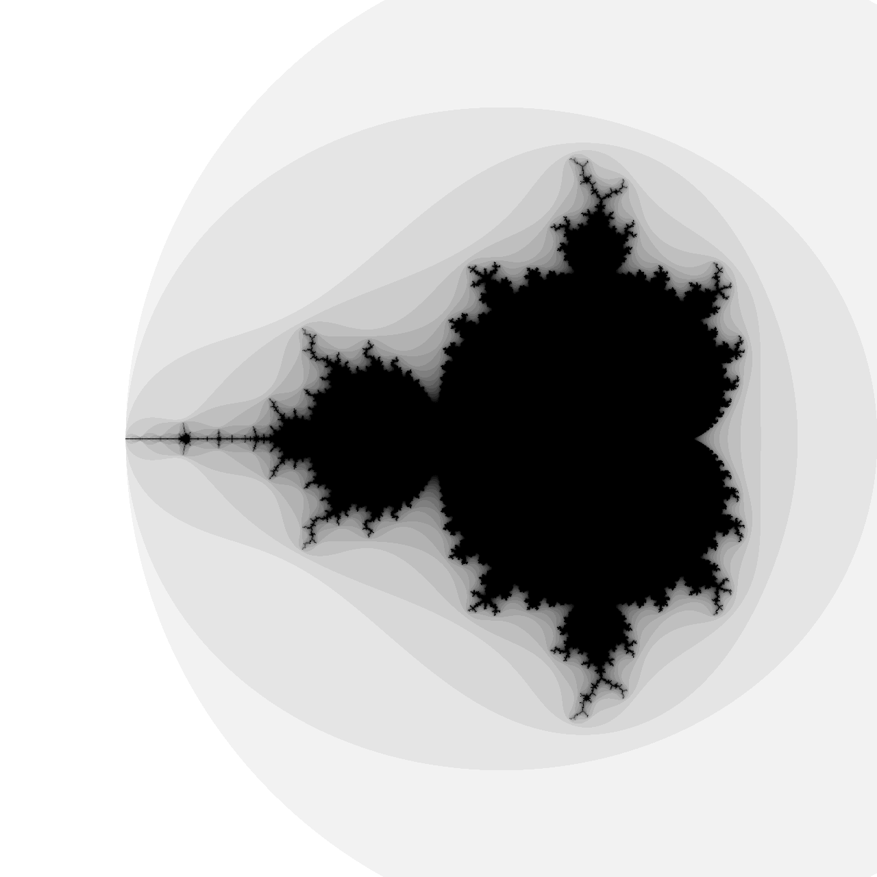
Whoa! That already looks way more interesting. Unfortunately, the stability values appear quantized at noticeably discrete levels because the escape count is an integer number. Increasing the maximum number of iterations can help alleviate that, but only to a certain extent. Besides, adding more iterations will filter out a lot of noise, leaving less content to see at this magnification level.
In the next subsection, you’ll learn about a better way of eliminating banding artifacts.
Smoothing Out the Banding Artifacts
Getting rid of color banding from the Mandelbrot set’s exterior boils down to using fractional escape counts. One way to interpolate their intermediate values is to use logarithms. The underlying math is quite involved, so let’s just take mathematicians’ word for it and update the code:
# mandelbrot.py

from dataclasses import dataclass
from math import log

@dataclass
class MandelbrotSet:
    max_iterations: int
    escape_radius: float = 2.0

    def __contains__(self, c: complex) -> bool:
        return self.stability(c) == 1

    def stability(self, c: complex, smooth=False) -> float:
        return self.escape_count(c, smooth) / self.max_iterations

    def escape_count(self, c: complex, smooth=False) -> int | float:
        z = 0
        for iteration in range(self.max_iterations):
            z = z ** 2 + c
            if abs(z) > self.escape_radius:
                if smooth:
                    return iteration + 1 - log(log(abs(z))) / log(2)
                return iteration
        return self.max_iterations
After importing the log() function from the math module, you add an optional Boolean flag that controls smoothing to your methods. When you turn the smoothing on, then math wizardry kicks in by combining the number of iterations with spatial information for the diverged number, spewing a floating-point number.
Note: The math formula above is based on the assumption that the escape radius approaches infinity, so it can’t be hardcoded anymore. That’s why your class now defines an optional escape_radius field with a default value of two, which you’ll be able to override at will when creating new instances of the MandelbrotSet.
Note that due to logarithms in your formula for the smoothed escape count, the associated stability can overshoot or even become negative! Here’s a quick example that demonstrates that:
>>> from mandelbrot import MandelbrotSet
>>> mandelbrot_set = MandelbrotSet(max_iterations=30)

>>> mandelbrot_set.stability(-1.2039 - 0.1996j, smooth=True)
1.014794475165942

>>> mandelbrot_set.stability(42, smooth=True)
-0.030071301713066417
Numbers greater than one and smaller than zero will lead to pixel intensities wrapping around the maximum and minimum levels allowed. So, don’t forget to clamp your scaled pixel values with max() and min() before lighting up a pixel:
# mandelbrot.py

from dataclasses import dataclass
from math import log

@dataclass
class MandelbrotSet:
    max_iterations: int
    escape_radius: float = 2.0

    def __contains__(self, c: complex) -> bool:
        return self.stability(c) == 1

    def stability(self, c: complex, smooth=False, clamp=True) -> float:
        value = self.escape_count(c, smooth) / self.max_iterations
        return max(0.0, min(value, 1.0)) if clamp else value

    def escape_count(self, c: complex, smooth=False) -> int | float:
        z = 0
        for iteration in range(self.max_iterations):
            z = z ** 2 + c
            if abs(z) > self.escape_radius:
                if smooth:
                    return iteration + 1 - log(log(abs(z))) / log(2)
                return iteration
        return self.max_iterations
When calculating the stability, you enable clamping by default but let the end-user decide how to deal with overflows and underflows. Some colorful visualizations might take advantage of this wrapping to produce interesting effects. This is controlled by the clamp flag in the .stability() method above. You’ll play around with visualizations in a later section.
Here’s how you can put your updated MandelbrotSet class into action:
>>> from mandelbrot import MandelbrotSet
>>> mandelbrot_set = MandelbrotSet(max_iterations=20, escape_radius=1000)

>>> width, height = 512, 512
>>> scale = 0.0075
>>> GRAYSCALE = "L"

>>> from PIL import Image
>>> image = Image.new(mode=GRAYSCALE, size=(width, height))
>>> for y in range(height):
...     for x in range(width):
...         c = scale * complex(x - width / 2, height / 2 - y)
...         instability = 1 - mandelbrot_set.stability(c, smooth=True)
...         image.putpixel((x, y), int(instability * 255))
...
>>> image.show()
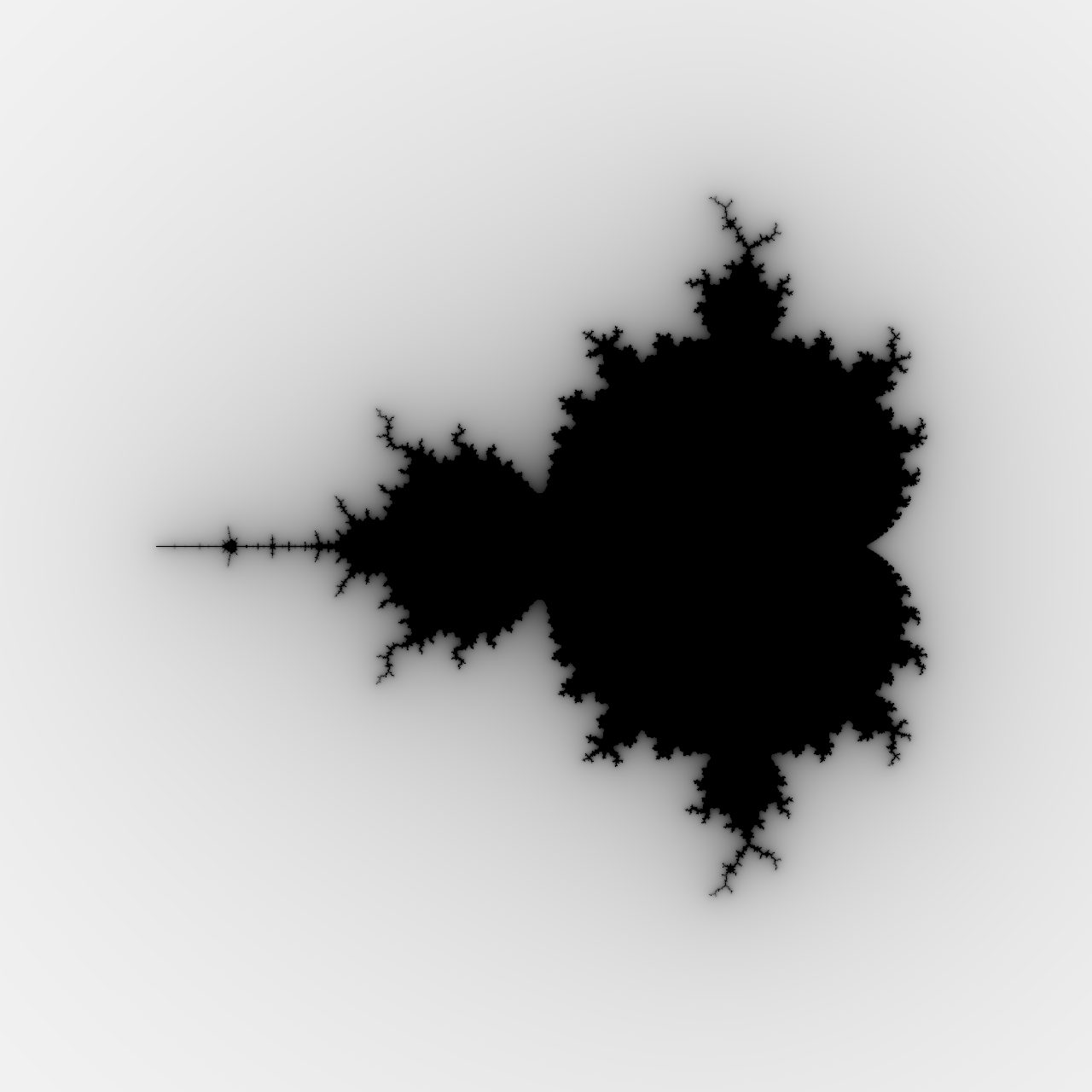
You enable smoothing by switching the smooth flag on for the stability calculation. However, doing only that would still produce a tiny bit of banding, so you may also increase the escape radius to a relatively large value such as one thousand. Finally, you’ll see a picture of the Mandelbrot set with a silky-smooth exterior:
Having fractional escape counts at your fingertips opens up interesting possibilities to play around with colors in your Mandelbrot set visualization. You’ll explore them later, but first, you can improve and streamline the drawing code to make it robust and more elegant.
Translating Between Set Elements and Pixels
So far, your visualization has depicted a static image of the fractal, but it hasn’t let you zoom in on a particular area or pan around to reveal more details. Unlike the logarithms before, the math for scaling and translating the image isn’t terribly difficult. However, it adds a bit of code complexity, which is worth abstracting away into helper classes before moving ahead.
On a high level, drawing the Mandelbrot set can be broken down into three steps:
- Convert a pixel’s coordinates into a complex number.
- Check if that complex number belongs to the Mandelbrot set.
- Assign a color to the pixel according to its stability.
You can build a smart pixel data type that’ll encapsulate the conversion between the coordinate systems, account for scaling, and handle the colors. For the integration layer between Pillow and your pixels, you can design a viewport class that’ll take care of panning and zooming.
The code for the Pixel and Viewport classes will follow soon, but once they’re implemented, you’ll be able to rewrite the drawing code in just a few lines of Python code:
>>> from PIL import Image
>>> from mandelbrot import MandelbrotSet
>>> from viewport import Viewport

>>> mandelbrot_set = MandelbrotSet(max_iterations=20)

>>> image = Image.new(mode="1", size=(512, 512), color=1)
>>> for pixel in Viewport(image, center=-0.75, width=3.5):
...     if complex(pixel) in mandelbrot_set:
...         pixel.color = 0
...
>>> image.show()
That’s it! The Viewport class wraps an instance of the Pillow’s image. It figures out the relevant scaling factor, offset, and the vertical extent of the world coordinates based on a center point and the viewport’s width in world units. As an iterable, it also supplies Pixel objects that you can loop through. Pixels know how to convert themselves into complex numbers, and they’re friends with the image instance wrapped by the viewport.
Note: The third argument passed to the constructor function of a Pillow’s image lets you set the background color, which defaults to black. In this case, you want a white background, which corresponds to pixel intensity equal to one in binary pixel mode.
You can implement the viewport by annotating it with the @dataclass decorator as you did with the MandelbrotSet class before:
# viewport.py

from dataclasses import dataclass
from PIL import Image

@dataclass
class Viewport:
    image: Image.Image
    center: complex
    width: float

    @property
    def height(self):
        return self.scale * self.image.height

    @property
    def offset(self):
        return self.center + complex(-self.width, self.height) / 2

    @property
    def scale(self):
        return self.width / self.image.width

    def __iter__(self):
        for y in range(self.image.height):
            for x in range(self.image.width):
                yield Pixel(self, x, y)
The viewport takes as arguments an image instance, a center point expressed as a complex number, and a horizontal span of world coordinates. It also derives a handful of read-only properties from those three parameters, which pixels will use later on. Finally, the class implements a special method, .__iter__(), which is part of the iterator protocol in Python that makes iteration over custom classes possible.
As you might have already guessed by looking at the code block above, the Pixel class accepts a Viewport instance and pixel coordinates:
# viewport.py (continued)

# ...

@dataclass
class Pixel:
    viewport: Viewport
    x: int
    y: int

    @property
    def color(self):
        return self.viewport.image.getpixel((self.x, self.y))

    @color.setter
    def color(self, value):
        self.viewport.image.putpixel((self.x, self.y), value)

    def __complex__(self):
        return (
                complex(self.x, -self.y)
                * self.viewport.scale
                + self.viewport.offset
        )
There’s only one property defined here, but it comprises both a getter and a setter for the pixel color, which delegate to Pillow through the viewport. The special method .__complex__() takes care of casting the pixel into a relevant complex number in world units. It flips the pixel coordinates along the vertical axis, converts them to a complex number, and then takes advantage of complex-numbers arithmetic in order to scale and move them.
Go ahead and give your new code a spin. The Mandelbrot set contains virtually limitless intricate structures that can only be seen under great magnification. Some areas feature spirals and zigzags resembling seahorses, octopuses, or elephants. As you zoom in, don’t forget to increase the maximum number of iterations to reveal more detail:
>>> from PIL import Image
>>> from mandelbrot import MandelbrotSet
>>> from viewport import Viewport

>>> mandelbrot_set = MandelbrotSet(max_iterations=256, escape_radius=1000)

>>> image = Image.new(mode="L", size=(512, 512))
>>> for pixel in Viewport(image, center=-0.7435 + 0.1314j, width=0.002):
...     c = complex(pixel)
...     instability = 1 - mandelbrot_set.stability(c, smooth=True)
...     pixel.color = int(instability * 255)
...
>>> image.show()
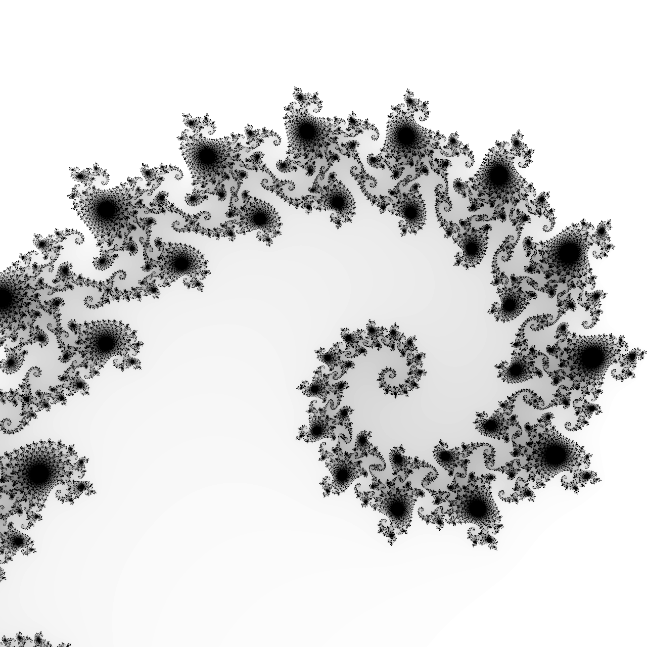
The viewport spans 0.002 world units and is centered at -0.7435 + 0.1314j, which is close to a Misiurewicz point that produces a beautiful spiral. Depending on the number of iterations, you’ll get a darker or brighter image with a varying degree of detail. You can use Pillow to increase the brightness if you feel like it:
>>> from PIL import ImageEnhance
>>> enhancer = ImageEnhance.Brightness(image)
>>> enhancer.enhance(1.25).show()
This will make the image brighter by 25% and display this spiral:
You can find many more unique points producing such spectacular results. Wikipedia hosts an entire image gallery of various details of the Mandelbrot set that are worth exploring.
If you’ve already started checking out different points, then you likely also noticed that the rendering time is highly sensitive to the area you’re currently looking at. Pixels located far from the fractal diverge to infinity sooner, while those closer to it tend to require more iterations. So, the more content there is in a specific area, the longer it takes to resolve if those pixels are stable or unstable.
There are some options available to you to improve the Mandelbrot set rendering performance in Python. However, they’re outside the scope of this tutorial, so feel free to explore them on your own if you’re curious. Now it’s time to give your fractal some color.
Making an Artistic Representation of the Mandelbrot Set
Since you can already draw the fractal in shades of gray, adding more colors shouldn’t be too difficult. It’s entirely up to you how to map a pixel’s stability into a hue. While there are many algorithms for plotting the Mandelbrot set in aesthetically pleasing ways, your imagination is the only limit!
If you haven’t been following along, then you can download the accompanying code by clicking the link below:
Get Source Code: Click here to get the source code you’ll use to draw the Mandelbrot set.
You’ll need to make a few adjustments to the drawing code from the previous section before moving on. Specifically, you’ll switch to a richer color mode and define a few reusable helper functions to make your life easier.
Color Palette
Artists have been mixing paints on a physical board called a palette since ancient times. In computing, a color palette represents a color lookup table, which is a form of lossless compression. It reduces the memory footprint of an image by indexing each individual color once and then referencing it in all the associated pixels.
This technique is relatively straightforward and fast to compute. Similarly, you can take a predefined palette to paint your fractal. However, rather than using pixel coordinates to find the corresponding color, you can use the escape count as the palette’s index. In fact, your earlier visualizations already did that by applying a palette of 256 monochrome grays, only without caching them in a lookup table.
To use more colors, you’ll need to create your image in the RGB mode first, which will allocate 24 bits per pixel:
image = Image.new(mode="RGB", size=(width, height))
From now on, Pillow will represent every pixel as a tuple comprised of the red, green, and blue (RGB) color channels. Each of the primary colors can take integers between 0 and 255, clocking in at a whopping 16.7 million unique colors. However, your color palettes will typically contain much fewer than that, in the neighborhood of the number of iterations.
Note: The number of colors in your palette doesn’t necessarily have to equal the maximum number of iterations. After all, it’s unknown how many stability values there’ll be until you run the recursive formula. When you enable smoothing, the number of fractional escape counts can be greater than the number of iterations!
If you’d like to test out a couple of different palettes, then it might be convenient to introduce a helper function to avoid retyping the same commands over and over again:
>>> from PIL import Image
>>> from mandelbrot import MandelbrotSet
>>> from viewport import Viewport

>>> def paint(mandelbrot_set, viewport, palette, smooth):
...     for pixel in viewport:
...         stability = mandelbrot_set.stability(complex(pixel), smooth)
...         index = int(min(stability * len(palette), len(palette) - 1))
...         pixel.color = palette[index % len(palette)]
The function takes a MandelbrotSet instance as an argument followed by Viewport, a color palette, and a smoothing flag. The color palette must be a list of tuples with the red, green, and blue channel values that Pillow expects. Notice that once you calculate a floating-point stability for the pixel at hand, you must scale it and clamp it before using it as an integer index in the palette.
Pillow only understands integers in the range of 0 through 255 for the color channels. However, working with normalized fractional values between 0 and 1 often prevents straining your brain. You may define another function that’ll reverse the normalization process to make the Pillow library happy:
>>> def denormalize(palette):
...     return [
...         tuple(int(channel * 255) for channel in color)
...         for color in palette
...     ]
This function scales fractional color values to integer ones. For example, it’ll convert a tuple with numbers like (0.13, 0.08, 0.21) to another tuple comprised of the following channel intensities: (45, 20, 53).
Coincidentally, the Matplotlib library includes several colormaps with such normalized color channels. Some colormaps are fixed lists of colors, while others are able to interpolate values given as a parameter. You can apply one of them to your Mandelbrot set visualization right now:
>>> import matplotlib.cm
>>> colormap = matplotlib.cm.get_cmap("twilight").colors
>>> palette = denormalize(colormap)

>>> len(colormap)
510
>>> colormap[0]
[0.8857501584075443, 0.8500092494306783, 0.8879736506427196]
>>> palette[0]
(225, 216, 226)
The twilight colormap is a list of 510 colors. After calling denormalize() on it, you’ll get a color palette suitable for your painting function. Before invoking it, you need to define a few more variables:
>>> mandelbrot_set = MandelbrotSet(max_iterations=512, escape_radius=1000)
>>> image = Image.new(mode="RGB", size=(512, 512))
>>> viewport = Viewport(image, center=-0.7435 + 0.1314j, width=0.002)
>>> paint(mandelbrot_set, viewport, palette, smooth=True)
>>> image.show()
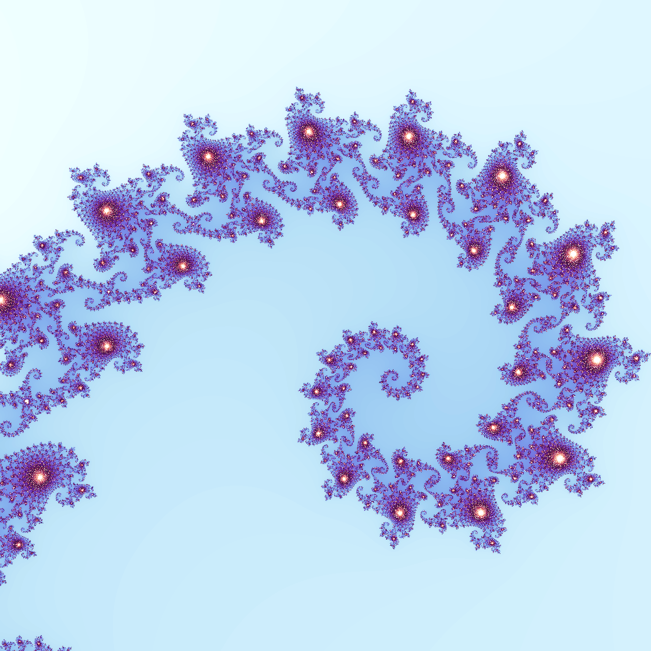
This will produce the same spiral as before but with a much more attractive appearance:
Feel free to try other color palettes included in Matplotlib or one of the third-party libraries that they mention in the documentation. Additionally, Matplotlib lets you reverse the color order by appending the _r suffix to a colormap’s name. You can also create a color palette from scratch, as shown below.
Suppose you wanted to emphasize the fractal’s edge. In such a case, you can divide the fractal into three parts and assign different colors to each:
>>> exterior = [(1, 1, 1)] * 50
>>> interior = [(1, 1, 1)] * 5
>>> gray_area = [(1 - i / 44,) * 3 for i in range(45)]
>>> palette = denormalize(exterior + gray_area + interior)
Choosing a round number for your palette, such as 100 colors, will simplify the formulas. Then, you can split the colors so that 50% goes to the exterior, 5% to the interior, and the remaining 45% to the gray area in between. You want both the exterior and interior to remain white by setting their RGB channels to fully saturated. However, the middle ground should gradually fade from white to black.
Don’t forget to set the viewport’s center point at -0.75 and its width to 3.5 units to cover the entire fractal. At this zoom level, you’ll also need to drop the number of iterations:
>>> mandelbrot_set = MandelbrotSet(max_iterations=20, escape_radius=1000)
>>> viewport = Viewport(image, center=-0.75, width=3.5)
>>> paint(mandelbrot_set, viewport, palette, smooth=True)
>>> image.show()
When you call paint() and show the image again, then you’ll see a clear boundary of the Mandelbrot set:
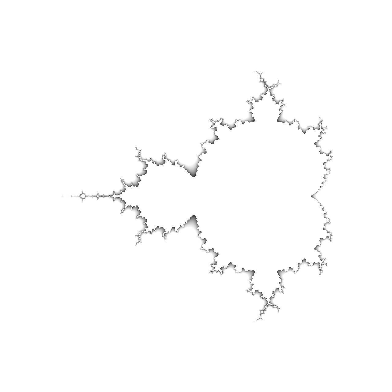
The continuous transition from white to black and then a sudden jump to pure white creates a shadowy embossing effect that brings out the edges of the fractal. Your color palette combines a few fixed colors with a smooth color progression known as a color gradient, which you’ll explore next.
Color Gradient
You may think of a gradient as a continuous color palette. The most common type of color gradient is the linear gradient, which uses linear interpolation for finding the closest value between two or more colors. You’ve just seen an example of such a color gradient when you mixed black and white to cast a shadow.
Now, you can work out the math for each gradient that you intend to use or build a universal gradient factory. Furthermore, if you’d like to distribute your colors in a non-linear fashion, then SciPy is your friend. The library comes with linear, quadratic, and cubic interpolation methods, among a few others. Here’s how you can take advantage of it:
>>> import numpy as np
>>> from scipy.interpolate import interp1d

>>> def make_gradient(colors, interpolation="linear"):
...     X = [i / (len(colors) - 1) for i in range(len(colors))]
...     Y = [[color[i] for color in colors] for i in range(3)]
...     channels = [interp1d(X, y, kind=interpolation) for y in Y]
...     return lambda x: [np.clip(channel(x), 0, 1) for channel in channels]
Your new factory function accepts a list of colors defined as triplets of floating-point values and an optional string with the name for the interpolation algorithm exposed by SciPy. The uppercase X variable contains normalized values between zero and one based on the number of colors. The uppercase Y variable holds three sequences of R, G, and B values for each color, and the channels variable has the interpolation functions for each channel.
When you call make_gradient() on some colors, then you’ll get a new function that’ll let you interpolate intermediate values:
>>> black = (0, 0, 0)
>>> blue = (0, 0, 1)
>>> maroon = (0.5, 0, 0)
>>> navy = (0, 0, 0.5)
>>> red = (1, 0, 0)

>>> colors = [black, navy, blue, maroon, red, black]
>>> gradient = make_gradient(colors, interpolation="cubic")

>>> gradient(0.42)
[0.026749999999999954, 0.0, 0.9435000000000001]
Note that gradient colors, such as black in the example above, can repeat and appear in any order. To hook up the gradient to your palette-aware painting function, you must decide on the number of colors in the corresponding palette and convert the gradient function to a fixed-sized list of denormalized tuples:
>>> num_colors = 256
>>> palette = denormalize([
...     gradient(i / num_colors) for i in range(num_colors)
... ])
...
>>> len(palette)
256
>>> palette[127]
(46, 0, 143)
You might feel tempted to use the gradient function directly against a stability value. Unfortunately, that would be computationally too expensive, pushing your patience to the limit. You want to compute the interpolation up front for all known colors instead of for every pixel.
Finally, after building the gradient factory, making a gradient function, and denormalizing the colors, you can paint the Mandelbrot set with your gradient palette:
>>> mandelbrot_set = MandelbrotSet(max_iterations=20, escape_radius=1000)
>>> paint(mandelbrot_set, viewport, palette, smooth=True)
>>> image.show()
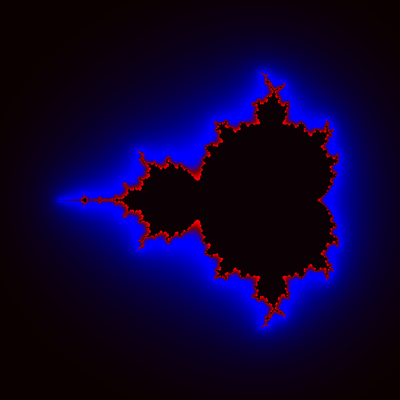
This will produce a glowing neon effect:
Keep increasing the number of iterations until you’re happy with the amount of smoothing and the number of details in the image. However, check out what comes next for the best results and the most intuitive way to manipulate colors.
Color Model
Up until now, you’ve been working in the realm of red, green, and blue (RGB) components, which isn’t the most natural way to think about colors. Fortunately, there are alternative color models that let you express the same concept. One is the Hue, Saturation, Brightness (HSB) color model, also known as Hue, Saturation, Value (HSV).
Note: Don’t confuse HSB or HSV with yet another color model: Hue, Saturation, Lightness (HSL).
Like RGB, the HSB model also has three components, but they’re different from the red, green, and blue channels. You can imagine an RGB color as a point enclosed in a three-dimensional cube. However, the same point has cylindrical coordinates in HSB:
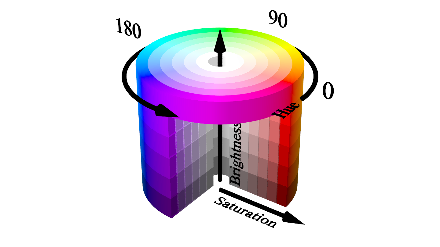
The three HSB coordinates are:
- Hue: The angle measured counterclockwise between 0° and 360°
- Saturation: The radius of the cylinder between 0% and 100%
- Brightness: The height of the cylinder between 0% and 100%
To use such coordinates in Pillow, you must translate them to a tuple of RGB values in the familiar range of 0 to 255:
>>> from PIL.ImageColor import getrgb

>>> def hsb(hue_degrees: int, saturation: float, brightness: float):
...     return getrgb(
...         f"hsv({hue_degrees % 360},"
...         f"{saturation * 100}%,"
...         f"{brightness * 100}%)"
...     )

>>> hsb(360, 0.75, 1)
(255, 64, 64)
Pillow already provides the getrgb() helper function that you can delegate to, but it expects a specially formatted string with the encoded HSB coordinates. On the other hand, your wrapper function takes hue in degrees and both saturation and brightness as normalized floating-point values. That makes your function compatible with stability values between zero and one.
There are a few ways in which you can associate stability with an HSB color. For example, you can use the entire spectrum of colors by scaling stability to 360° degrees, use the stability to modulate the saturation, and set the brightness to 100%, which is indicated by 1 below:
>>> mandelbrot_set = MandelbrotSet(max_iterations=20, escape_radius=1000)
>>> for pixel in Viewport(image, center=-0.75, width=3.5):
...     stability = mandelbrot_set.stability(complex(pixel), smooth=True)
...     pixel.color = (0, 0, 0) if stability == 1 else hsb(
...         hue_degrees=int(stability * 360),
...         saturation=stability,
...         brightness=1,
...     )
...
>>> image.show()
To paint the interior black, you check that the stability of a pixel is exactly one and set all three color channels to zero. For stability values less than one, the exterior will have a saturation that fades with distance from the fractal and a hue that follows the HSB cylinder’s angular dimension:
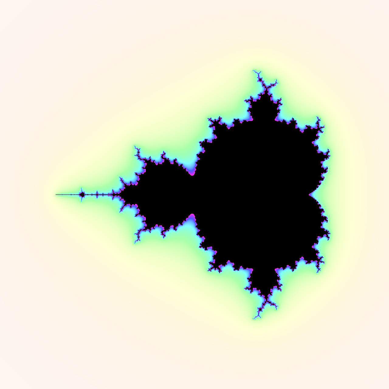
The angle increases as you get closer to the fractal, changing colors from yellow through green, cyan, blue, and magenta. You can’t see the red color because the fractal’s interior is always painted black, while the furthest part of the exterior has little saturation. Note that rotating the cylinder by 120° allows you to locate each of the three primary colors (red, green, and blue) on its base.
Don’t hesitate to experiment with calculating the HSB coordinates in different ways and see what happens!
Conclusion
Now you know how to use Python to plot and draw the famous fractal discovered by Benoît Mandelbrot. You’ve learned various ways of visualizing it with colors as well as in grayscale and black and white. You’ve also seen a practical example illustrating how complex numbers can help elegantly express a mathematical formula in Python.
In this tutorial, you learned how to:
- Apply complex numbers to a practical problem
- Find members of the Mandelbrot and Julia sets
- Draw these sets as fractals using Matplotlib and Pillow
- Make a colorful artistic representation of the fractals
You can download the complete source code used throughout this tutorial by clicking the link below:
Get Source Code: Click here to get the source code you’ll use to draw the Mandelbrot set.