Python 3.15 ships with a brand-new profiling package defined in PEP 799. It finally retires the ancient profile module, gives cProfile a new home under profiling.tracing, and adds profiling.sampling, a statistical sampling profiler code-named Tachyon. You can point it at a script, a module, or even a live production process, and it’ll tell you where the time goes with virtually no overhead.
By the end of this tutorial, you’ll understand that:
- Python 3.15 organizes its profilers under a new
profilingpackage, deprecating the oldprofilemodule. - The new sampling profiler peeks at your program’s call stack from the outside, so your code runs at full speed while being profiled.
- You can attach to a running process by its PID without restarting or modifying the target, as long as you have the right permissions.
- Sampling modes let you separate CPU work from I/O waits and isolate code that runs while holding the GIL or handling an exception.
- The profiler supports many output formats, including interactive flame graphs, line-level heatmaps, and a live top-like terminal dashboard.
First, you’ll get a quick refresher on how tracing and sampling profilers differ. Then, you’ll set up Python 3.15 with uv and profile a small 3D renderer with deliberately planted bottlenecks. Along the way, you’ll try out threads, async tasks, native-code boundaries, and the visualizations the profiler offers.
To get the most out of this tutorial, you should be comfortable running commands in a terminal because that’s where the profiler lives. It’ll also help if you’ve dabbled in threading or asyncio before, as you’ll profile both kinds of concurrency. Prior profiling experience is a plus, not a requirement. You’ll review the essential theory as you go.
Note: The examples in this tutorial use Python 3.15.0b4, so some details may shift slightly before the final release in October.
Get Your Code: Click here to download the free sample code you’ll use to explore the sampling profiler in Python 3.15.
Take the Quiz: Test your knowledge with our interactive “Python 3.15 Preview: Sampling Profiler” quiz. You’ll receive a score upon completion to help you track your learning progress:
Interactive Quiz
Python 3.15 Preview: Sampling ProfilerTest your understanding of Python 3.15's new sampling profiler, from CPU and GIL modes to flame graphs, heatmaps, and attaching to a live process.
Get to Know Python’s New profiling Package
For decades, Python has shipped two deterministic profilers in the standard library:
The first one is a pure-Python implementation that’s mostly of educational value, while the second one does the same job in the C programming language at a fraction of the cost. PEP 799 tidies up this corner in Python 3.15 by introducing a dedicated profiling package with two submodules:
| Module | What It Is |
|---|---|
profiling.tracing |
The deterministic tracing profiler formerly known as cProfile |
profiling.sampling |
The new statistical sampling profiler, code-named Tachyon |
The old modules don’t disappear overnight, though. The cProfile module sticks around indefinitely as a thin alias, so your existing tooling won’t break. On the other hand, the pure-Python profile module enters its retirement. Importing it now triggers a warning, and Python 3.17 will remove it entirely:
>>> import profile
<python-input-0>:1: DeprecationWarning: The profile module is deprecated
⮑ and will be removed in Python 3.17. Use profiling.tracing (or cProfile)
⮑ for tracing profilers instead.

>>> import cProfile
>>> import profiling.tracing
>>> cProfile.Profile is profiling.tracing.Profile
True
The comparison in the last line proves that cProfile and profiling.tracing expose the very same class, so the two names are interchangeable. If you’d like a refresher on using the tracing profiler and interpreting its output, then check out Profiling in Python, which walks through cProfile and friends in detail.
The package reorganization in the standard library is the boring part of PEP 799. The interesting part is profiling.sampling, and that’s what you’ll spend the rest of this tutorial on.
Compare Tracing and Sampling Profilers
Before you fire up the new sampling profiler, it helps to know how it differs from its tracing counterpart. Both tools answer the same question, namely where your program spends most of its time. They just gather evidence in different ways. That difference dictates when you should reach for each of them. Here’s the thirty-second version of the theory before you dive deeper.
How Tracing Profilers Work
A deterministic tracing profiler hooks into the interpreter and registers a callback that runs on every single function call and return. Nothing escapes it. The resulting numbers are exact, down to how many times each function ran.
You can watch this happen below. Press play, and the profiler fires a hook on every call and return of a small demo program:
That precision comes at a price. The constant interruptions can slow your program down severalfold and, worse, distort the measurements themselves. Cheap functions called millions of times suddenly look expensive because the profiler’s bookkeeping dwarfs their actual work. That’s why running a tracing profiler against a production workload is rarely an option.
How Sampling Profilers Work
A statistical sampling profiler takes the opposite approach. Instead of instrumenting your code, it periodically captures snapshots of the call stack—by default, a thousand times per second—and counts which functions it catches in the act. Functions that consume the most time will statistically appear in the most samples.
The companion visualization runs the same program at full speed while probes sample the stack at a fixed interval. Press play, and then drag the interval slider to sample more or less often:
Give the faster probe rates a try, and watch the statistics converge. At the default thousand samples per second, the tiny log() calls slip between the probes. Crank up the rate, and the sampled shares settle on the same 96 percent and 4 percent that the tracing profiler measured, while the run time still shows no slowdown. With enough samples, the sampling profiler’s results approach the tracing profiler’s, but with far less overhead.
What sets Python 3.15’s implementation apart is that it captures those stack snapshots from a separate process, reading the target’s memory directly through operating system APIs. Your program doesn’t run a single extra bytecode instruction. It’s never paused, patched, or even aware that it’s being watched, which makes the new profiler safe to point at production workloads.
The trade-off is precision. A sampler can miss short-lived functions entirely, and it can’t tell you how many times a function was called. In practice, that’s a great deal because you rarely optimize anything but the functions that dominate the profile anyway.
When to Use Which
Here’s a rule of thumb that you can use to pick the right profiler for each situation:
| Situation | Tracing | Sampling |
|---|---|---|
| Short-running script or test on your laptop | ✅ | |
| Exact call counts needed | ✅ | |
| Long-running service, GUI app, or production job | ✅ | |
| Minimal overhead or attach-to-live-process needed | ✅ |
Sampling profilers for Python aren’t a new idea. Third-party tools like Austin, py-spy, and pyinstrument have offered external sampling for years, and Python 3.12 taught the Linux perf profiler to understand Python frames. What’s new is having a capable, officially supported sampler in every Python installation, maintained by the core team and aware of the interpreter’s internals.
Take Python 3.15’s Sampling Profiler for a Spin
That’s enough theory for now. In this section, you’ll grab a pre-release version of Python 3.15 and get familiar with the demo project that you’ll be profiling for the rest of this tutorial. You’ll also run your first profiles—one to find the hottest function and another to prove that it spends its time waiting rather than working.
Set Up Python 3.15 With uv
Because Python 3.15 won’t reach its final release until October, you’ll need a pre-release build. The quickest path is uv, which manages Python versions for you. The sample project for this tutorial is called Pretzel and requires at least Python 3.15 in its pyproject.toml, so a single command inside the project folder fetches a pre-built CPython 3.15 and assembles a virtual environment:
$ cd materials-python315-sampling-profiler/
$ uv sync
Using CPython 3.15.0b4
Creating virtual environment at: .venv
Resolved 2 packages in 0.78ms
Installed 2 packages in 13ms
 + numpy==2.5.1
 + pretzel==0.1.0 (from file:///.../materials-python315-sampling-profiler)
$ uv run python -VV
Python 3.15.0b4 (main, Jul 18 2026, 17:04:20) [Clang 22.1.3 ]
That’s the entire setup. Once 3.15 goes final, the same command will pick up the stable release instead of the beta.
The project you just installed is a tiny 3D model viewer written mostly in pure Python with a pinch of NumPy. It loads a trefoil knot from a pretzel.mdl file, shades it with simulated ambient light sampled from a background image, and spins it in a Tkinter window.
You can start the animation with uv run pretzel:
Alternatively, you can render a fixed number of frames headlessly. In headless mode, the application performs all its usual processing and computation but never displays a window on the screen. Skipping the display removes a source of variability, making the workload identical from one run to the next, which is perfect for repeatable profiling runs:
$ uv run pretzel --frames 300
Rendered 300 frames in 5.95s (50.4 fps)
The exact numbers you see may differ from the ones shown in this tutorial. Frame rates depend on your hardware and overall system load. But that’s okay. What matters is the relative picture, such as how the profiled run compares to the unprofiled one, and which functions rise to the top.
Pretzel looks innocent, but it hides four performance problems for you to uncover, each designed to exercise a different profiler feature:
- A pure-Python hotspot in the geometry pipeline that transforms, culls, sorts, and assembles thousands of triangles per frame
- A native-code hotspot in the NumPy-based lighting calculations
- An I/O-bound bottleneck that flushes telemetry to disk after every frame
- A wasteful parser that decodes background images one byte at a time in a worker thread
Time to find them all!
Profile a Whole Program Run
The profiler lives behind the profiling.sampling module, which you can run directly from your terminal:
$ uv run python -m profiling.sampling
usage: python3 -m profiling.sampling [-h] {run,attach,dump,replay} ...
python3 -m profiling.sampling: error: the following arguments are required: command
Running the module without any arguments prints a usage message because the profiler needs to know what you want it to do. Its command-line interface groups the available functionality into four subcommands:
| Subcommand | Description |
|---|---|
run |
Run and profile a script or module |
attach |
Attach to and profile a running process |
dump |
Dump a running process’s current stack |
replay |
Replay a binary profile and convert to another format |
You’ll start with run, which launches a Python script or module and profiles it from the first line to the last. While the exact frame rate may look different for you, the profiled run should land close to the unprofiled one, and the hottest lines should point at the same handful of functions:
$ uv run python -m profiling.sampling run -m pretzel --frames 300
Rendered 300 frames in 6.10s (49.2 fps)
Captured 6,516 samples in 6.52 seconds
Sample rate: 1,000.00 samples/sec
Error rate: 1.89
Profile Stats:
       nsamples   sample%   tottime (s)    cumul%   cumtime (s)  filename:lineno(function)
      1331/1331      20.8         1.331      20.8         1.331  telemetry.py:15(FrameLog.record)
        711/711      11.1         0.711      11.1         0.711  render.py:46(compute_frame)
        494/494       7.7         0.494       7.7         0.494  shading.py:30(shade_faces)
        436/436       6.8         0.436       6.8         0.436  _methods.py:132(_mean)
        353/353       5.5         0.353       5.5         0.353  shading.py:29(shade_faces)
        250/250       3.9         0.250       3.9         0.250  render.py:42(compute_frame)
        224/224       3.5         0.224       3.5         0.224  engine.py:72(cull_backfaces)
        177/177       2.8         0.177       2.8         0.177  shading.py:37(shade_faces)
       173/4700       2.7         0.173      73.5         4.700  cli.py:56(render_headlessly)
        166/166       2.6         0.166       2.6         0.166  render.py:47(compute_frame)
        146/241       2.3         0.146       3.8         0.241  engine.py:84(sort_back_to_front)
         90/117       1.4         0.090       1.8         0.117  engine.py:61(project_vertices)
         84/573       1.3         0.084       9.0         0.573  shading.py:22(sample_ambient_light)
          84/84       1.3         0.084       1.3         0.084  numeric.py:1712(cross)
          81/81       1.3         0.081       1.3         0.081  engine.py:49(transform_vertices)
(...)
Notice that the app rendered at 49.2 frames per second under the profiler, compared to roughly 50 without it. There’s no instrumentation slowing the interpreter down. The profiler runs in a separate process, so the only cost is a bit of competition for CPU cores.
Note: The sampling profiler reads the target process’s memory, which most operating systems restrict:
- Linux: The
runcommand works out of the box because the profiler spawns your program as a child process, and the default Linux kernel security setting (ptrace_scope=1) permits a parent to trace its own children. - macOS: Prefix the command with
sudo -Eto preserve your environment, as the profiler calls the low-level macOS kernel functiontask_for_pid(), which hands out a handle to another process’s memory and requires elevated privileges. Additionally, System Integrity Protection (SIP) blocks access to system Python binaries even with elevated privileges, so stick to a user-installed interpreter like the oneuvprovides. - Windows: Use an elevated shell and run the profiler from your global Python installation rather than a virtual environment because the venv’s
python.exeis only a launcher shim that re-executes the real interpreter as a child process.
In short, run needs no special setup on Linux, but macOS and Windows require elevated privileges. You’ll encounter these restrictions again with attach, which has stricter requirements on all three platforms.
The header tells you that the profiler collected 6,516 samples at the default rate of one thousand per second. The error rate is the percentage of snapshot attempts that got discarded because the target’s call stack mutated mid-read. Since the target never stops running, an occasional torn read is expected, and the profiler just drops those samples.
Each row then describes one location in your code using the pstats format. The legend printed below the table explains the meaning of each column:
- nsamples: Direct/cumulative samples (direct executing / on call stack)
- sample%: Percentage of total samples this function was directly executing
- tottime: Estimated total time spent directly in this function
- cumul%: Percentage of total samples when this function was on the call stack
- cumtime: Estimated cumulative time (including time in called functions)
- filename:lineno(function): Function location and name
The first column shows the number of direct samples and cumulative samples. In other words, it tells you how often the function was caught directly executing at the top of the call stack, versus how often it was anywhere on the stack. For example, 84/573 next to sample_ambient_light() means the function was on the stack in 573 samples but personally doing the work in only 84 of them.
The last column identifies not just the function but the exact line that was executing. That’s why compute_frame() and shade_faces() each appear several times. The profiler resolves samples down to individual lines.
By default, the profiler also prints a summary of interesting functions, grouping the usual suspects for you:
Functions with Highest Direct/Cumulative Ratio (Hot Spots):
  1.000 direct/cumulative ratio, 20.8% direct samples: telemetry.py:(FrameLog.record)
  1.000 direct/cumulative ratio, 17.6% direct samples: render.py:(compute_frame)
  1.000 direct/cumulative ratio, 16.0% direct samples: shading.py:(shade_faces)

Functions with Highest Call Frequency (Indirect Calls):
  4527 indirect calls, 73.5% total stack presence: cli.py:(render_headlessly)
  489 indirect calls, 9.0% total stack presence: shading.py:(sample_ambient_light)
  95 indirect calls, 3.8% total stack presence: engine.py:(sort_back_to_front)

Functions with Highest Call Magnification (Cumulative/Direct):
  27.2x call magnification, 4527 indirect calls from 173 direct: cli.py:(render_headlessly)
  6.8x call magnification, 489 indirect calls from 84 direct: shading.py:(sample_ambient_light)
  1.7x call magnification, 95 indirect calls from 146 direct: engine.py:(sort_back_to_front)
The verdict so far is that the single hottest line in the program is FrameLog.record() in telemetry.py, which writes one frame’s statistics to a log file. That’s suspicious for such a cheap operation.
Note: How prominently the telemetry writer shows up depends on your file system and drive. On fast storage, the call that forces data to disk can return before the data actually reaches the physical media, so the write may barely register. If FrameLog.record() doesn’t top your table, don’t worry. The rest of the tutorial still holds.
You can tweak the report with --sort, limit it with --limit, or silence the extras with --no-summary. To see all the knobs, including -r for the sampling rate, run the following command:
$ uv run python -m profiling.sampling run --help
No matter how you tweak the report, one line stands out and calls for an explanation. Why should writing a handful of bytes to a log file cost more than transforming thousands of triangles? To answer that, you’ll need to look at the same run through a different lens.
Split Wall-Clock Time From CPU Time
By default, the profiler samples in wall-clock mode, counting every moment the code sits on the call stack, whether it’s crunching numbers or waiting for the disk. The --mode option changes that lens. Rerun the profile in CPU mode, which counts samples only while the thread actually runs on a CPU core:
$ uv run python -m profiling.sampling run --mode cpu -m pretzel --frames 300
Rendered 300 frames in 6.14s (48.9 fps)
Captured 6,562 samples in 6.56 seconds
Sample rate: 1,000.00 samples/sec
Error rate: 2.19
Profile Stats:
       nsamples   sample%  tottime (ms)    cumul%   cumtime (s)  filename:lineno(function)
        705/705      15.4       705.000      15.4         0.705  render.py:46(compute_frame)
        404/404       8.8       404.000       8.8         0.404  shading.py:30(shade_faces)
        366/366       8.0       366.000       8.0         0.366  _methods.py:132(_mean)
        338/338       7.4       338.000       7.4         0.338  shading.py:29(shade_faces)
(...)
The telemetry writer that topped the previous chart has vanished from the leaderboard. Its place at the top now belongs to line 46 of render.py, which formats polygon colors. It’s pure CPU work that you’ll fix later with the help of a differential flame graph.
More importantly, when a bottleneck dominates in wall-clock mode but disappears in CPU mode, you’ve caught your program waiting rather than working. In this case, the culprit is a classic:
src/pretzel/telemetry.py
 2"""Record per-frame timings to a log file that survives crashes."""
 3
 4import os
 5
 6class FrameLog:
 7    def __init__(self, path: str, durable: bool = True) -> None:
 8        self.durable = durable
 9        self._file = open(path, "w", encoding="utf-8")
10
11    def record(self, frame: int, elapsed_ms: float) -> None:
12        self._file.write(f"{frame},{elapsed_ms:.3f}\n")
13        if self.durable:
14            self._file.flush()
15            os.fsync(self._file.fileno())
16
17    def close(self) -> None:
18        self._file.close()
Pretzel calls os.fsync() after rendering every frame, forcing the operating system to flush its write buffers all the way to the physical disk. That’s a few milliseconds of dead air, dozens of times per second. It’s an I/O-bound bottleneck, so it costs wall-clock time, not CPU time.
Here’s the kicker. Pretzel’s own frame timer never notices because the log entry gets written after the measurement ends. The app happily reports fourteen milliseconds per frame in telemetry.csv while delivering a frame only every twenty milliseconds. Your instrumentation can lie to you, but an external profiler that watches the whole process can’t be fooled so easily.
Beyond wall-clock (the default) and CPU mode, there are two more worth exploring:
--mode gil: Counts only samples where the thread holds the Global Interpreter Lock.--mode exception: Counts only samples taken while an exception is in flight.
You’ll see the GIL mode in action next.
Profile Threads, Async Tasks, and Native Code
Real programs rarely run as a single thread of pure Python. Work spreads across worker threads, asyncio tasks, and compiled extension modules. Each of those is a place where naive profiles tend to mislead. The profiler has a dedicated answer for all three, and Pretzel gives you a chance to try each one.
Watch Your Threads Fight for the GIL
So far, the profiler has watched only the main thread, as it does by default. Pretzel, however, runs a second thread that periodically hot-reloads the background image. Add -a (short for --all-threads) to sample every thread in the process:
$ uv run python -m profiling.sampling run -a -m pretzel --frames 300
Rendered 300 frames in 6.05s (49.6 fps)
Captured 6,466 samples in 6.47 seconds
Sample rate: 999.94 samples/sec
Error rate: 2.81
Profile Stats:
       nsamples   sample%   tottime (s)    cumul%   cumtime (s)  filename:lineno(function)
      5293/5293      43.3         5.293      43.3         5.293  streaming.py:30(BackgroundStreamer.run)
      1268/1268      10.4         1.268      10.4         1.268  telemetry.py:15(FrameLog.record)
        703/703       5.7         0.703       5.7         0.703  render.py:46(compute_frame)
        525/525       4.3         0.525       4.3         0.525  _methods.py:132(_mean)
        420/420       3.4         0.420       3.4         0.420  shading.py:30(shade_faces)
        341/341       2.8         0.341       2.8         0.341  shading.py:29(shade_faces)
        242/242       2.0         0.242       2.0         0.242  render.py:42(compute_frame)
        224/224       1.8         0.224       1.8         0.224  assets.py:56(decode_ppm_pixel_by_pixel)
        215/351       1.8         0.215       2.9         0.351  assets.py:53(decode_ppm_pixel_by_pixel)
        202/202       1.7         0.202       1.7         0.202  engine.py:72(cull_backfaces)
       186/4654       1.5         0.186      38.0         4.654  cli.py:56(render_headlessly)
        168/168       1.4         0.168       1.4         0.168  render.py:47(compute_frame)
        144/144       1.2         0.144       1.2         0.144  shading.py:37(shade_faces)
        141/185       1.2         0.141       1.5         0.185  assets.py:51(decode_ppm_pixel_by_pixel)
        140/140       1.1         0.140       1.1         0.140  assets.py:78(to_linear)
(...)
A whole new thread’s worth of samples appears, led by BackgroundStreamer.run(). Don’t panic at the 43.3 percent, though. Line 30 of streaming.py is a time.sleep() call, so the streamer thread spends most of its life idling between reloads. Also, keep in mind that with --all-threads, each sample can now capture several stacks at once, so the reported times add up to thread-seconds, which can exceed the wall-clock duration of the run.
The more interesting rows belong to decode_ppm_pixel_by_pixel(), the deliberately wasteful image parser that reads a background image byte by byte. Sleeping threads are harmless, but this one might not be while it’s awake. Python threads share a single interpreter, so ask the profiler who’s hogging the GIL:
$ uv run python -m profiling.sampling run --mode gil -a -m pretzel --frames 300
Rendered 300 frames in 6.05s (49.6 fps)
Captured 6,463 samples in 6.46 seconds
Sample rate: 1,000.00 samples/sec
Error rate: 2.58
Profile Stats:
       nsamples   sample%  tottime (ms)    cumul%   cumtime (s)  filename:lineno(function)
        724/724      16.5       724.000      16.5         0.724  render.py:46(compute_frame)
        354/354       8.1       354.000       8.1         0.354  shading.py:30(shade_faces)
        344/344       7.8       344.000       7.8         0.344  shading.py:29(shade_faces)
        226/226       5.2       226.000       5.2         0.226  render.py:42(compute_frame)
        221/221       5.0       221.000       5.0         0.221  assets.py:56(decode_ppm_pixel_by_pixel)
        212/327       4.8       212.000       7.5         0.327  assets.py:53(decode_ppm_pixel_by_pixel)
        194/194       4.4       194.000       4.4         0.194  engine.py:72(cull_backfaces)
       181/3417       4.1       181.000      77.9         3.417  cli.py:56(render_headlessly)
        170/189       3.9       170.000       4.3         0.189  assets.py:51(decode_ppm_pixel_by_pixel)
        144/144       3.3       144.000       3.3         0.144  render.py:47(compute_frame)
        137/239       3.1       137.000       5.4         0.239  engine.py:84(sort_back_to_front)
        129/129       2.9       129.000       2.9         0.129  shading.py:37(shade_faces)
        122/122       2.8       122.000       2.8         0.122  assets.py:78(to_linear)
        110/132       2.5       110.000       3.0         0.132  engine.py:61(project_vertices)
          85/85       1.9        85.000       1.9         0.085  engine.py:82(sort_back_to_front.<locals>.face_depth)
(...)
In GIL mode, all the sleeping and disk-flushing evaporates, leaving only the code that holds the interpreter hostage. The parser claims about 13.7 percent of all GIL time, which is real contention. Whenever the streamer decodes a background image, the renderer must wait for the lock, and the animation stutters.
On a free-threaded build, this mode loses its meaning, but on the default build, it’s the quickest way to diagnose why your multithreaded program won’t scale.
Profile Async Code Task by Task
Threads aren’t the only concurrency story in Python. If you profile an asyncio program naively, then you’ll mostly discover that the event loop waits a lot. The sample project ships with a small script that concurrently downloads three fake textures and then decodes them. The CATALOG constant maps their names to simulated latencies:
examples/fetch_textures.py
"""Download and decode textures concurrently with asyncio."""

import asyncio

CATALOG = {
    "bakery-dawn": 0.35,
    "bakery-noon": 0.15,
    "bakery-dusk": 0.25,
}

async def download_texture(name: str, latency: float) -> bytes:
    await asyncio.sleep(latency)
    return name.encode() * 100_000

async def decode_texture(payload: bytes) -> int:
    checksum = 0
    for byte in payload:
        checksum = (checksum * 31 + byte) % 1_000_003
    return checksum

async def main() -> None:
    async with asyncio.TaskGroup() as group:
        downloads = {
            name: group.create_task(
                download_texture(name, latency), name=f"download-{name}"
            )
            for name, latency in CATALOG.items()
        }
    for name, download in downloads.items():
        checksum = await decode_texture(download.result())
        print(f"{name}: {checksum}")

if __name__ == "__main__":
    asyncio.run(main())
Profile it the regular way, and the top of the chart is dominated by EpollSelector.select() at roughly 60 percent. That’s the event loop twiddling its thumbs, telling you nothing about your coroutines. The --async-aware flag fixes that by reconstructing logical stacks from task boundaries instead of showing raw interpreter frames:
$ uv run python -m profiling.sampling run --async-aware \
    examples/fetch_textures.py
bakery-dawn: 142978
bakery-noon: 336182
bakery-dusk: 982760
Captured 605 samples in 0.61 seconds
Sample rate: 1,000.00 samples/sec
Error rate: 0.00
Profile Stats:
       nsamples   sample%  tottime (ms)    cumul%  cumtime (ms)  filename:lineno(function)
        180/180      91.4       180.000      91.4       180.000  fetch_textures.py:20(decode_texture)
          12/12       6.1        12.000       6.1        12.000  fetch_textures.py:19(decode_texture)
            5/5       2.5         5.000       2.5         5.000  fetch_textures.py:14(download_texture)
            0/2       0.0         0.000       1.0         2.000  <task>:0(download-bakery-noon)
            0/5       0.0         0.000       2.5         5.000  taskgroups.py:124(TaskGroup._aexit)
            0/5       0.0         0.000       2.5         5.000  taskgroups.py:75(TaskGroup.__aexit__)
            0/5       0.0         0.000       2.5         5.000  fetch_textures.py:25(main)
          0/197       0.0         0.000     100.0       197.000  <task>:0(Task-1)
            0/2       0.0         0.000       1.0         2.000  <task>:0(download-bakery-dusk)
            0/1       0.0         0.000       0.5         1.000  <task>:0(download-bakery-dawn)
          0/192       0.0         0.000      97.5       192.000  fetch_textures.py:33(main)
(...)
Now the checksum loop in decode_texture() stands out as the real CPU consumer. By default, async-aware profiling counts only the task that’s currently running. Add --async-mode all to also sample tasks that are suspended at an await expression:
$ uv run python -m profiling.sampling run --async-aware --async-mode all \
    examples/fetch_textures.py
bakery-dawn: 142978
bakery-noon: 336182
bakery-dusk: 982760
Captured 590 samples in 0.59 seconds
Sample rate: 1,000.00 samples/sec
Error rate: 0.00
Profile Stats:
       nsamples   sample%  tottime (ms)    cumul%  cumtime (ms)  filename:lineno(function)
        751/751      79.4       751.000      79.4       751.000  tasks.py:704(sleep)
        192/192      20.3       192.000      20.3       192.000  fetch_textures.py:33(main)
            1/1       0.1         1.000       0.1         1.000  fetch_textures.py:24(main)
          1/351       0.1         1.000      37.1       351.000  <task>:0(download-bakery-dawn)
            1/1       0.1         1.000       0.1         1.000  fetch_textures.py:14(download_texture)
          0/946       0.0         0.000     100.0       946.000  <task>:0(Task-1)
          0/751       0.0         0.000      79.4       751.000  fetch_textures.py:13(download_texture)
          0/252       0.0         0.000      26.6       252.000  <task>:0(download-bakery-dusk)
          0/753       0.0         0.000      79.6       753.000  taskgroups.py:124(TaskGroup._aexit)
          0/753       0.0         0.000      79.6       753.000  taskgroups.py:75(TaskGroup.__aexit__)
          0/753       0.0         0.000      79.6       753.000  fetch_textures.py:25(main)
          0/150       0.0         0.000      15.9       150.000  <task>:0(download-bakery-noon)
(...)
The synthetic <task> frames now itemize where each task spent its life waiting, and because the script names its tasks with group.create_task(…, name=…), you can tell your downloads apart at a glance. Naming your tasks was always good hygiene, and now it pays off in profiles, too.
Note that --async-aware can’t be combined with --all-threads, --native, --no-gc, or any mode other than the default wall-clock one.
See Where Python Hands Off to Native Code
One of Pretzel’s bottlenecks hides in shading.py, where NumPy computes the lighting. Look back at the very first profile. Lines 29 and 30 of shade_faces() rank high even though each one is a single NumPy expression:
src/pretzel/shading.py
24# ...
25
26def shade_faces(
27    faces: list[Face], transformed: list[Vertex], ambient: float
28) -> list[list[int]]:
29    vertices = np.asarray(transformed)
30    corners = vertices[np.asarray(faces)]
31    edges_ab = corners[:, 1] - corners[:, 0]
32    edges_ac = corners[:, 2] - corners[:, 0]
33    normals = np.cross(edges_ac, edges_ab)
34    normals /= np.linalg.norm(normals, axis=1, keepdims=True)
35    diffuse = np.clip(normals @ LIGHT_DIRECTION, 0.0, 1.0)
36    intensity = np.clip(ambient + (1.0 - ambient) * diffuse, 0.0, 1.0)
37    return (CRUST_COLOR * intensity[:, np.newaxis]).astype(np.uint8).tolist()
When the interpreter dives into a C extension, the sampler can’t see beyond the last Python frame, so all that native time gets billed to the calling line.
That attribution can be slightly misleading. Those lines aren’t slow Python. Instead, they’re busy C code. To make the boundary explicit, pass --native, and the profiler will insert artificial <native> frames wherever the interpreter has handed control to compiled code.
The quickest way to see them is the dump subcommand, which snapshots the current stack of a live process. The --blocking flag briefly pauses the target for a perfectly consistent snapshot, and sudo grants the debugger-level access that you’ll learn more about when attaching to a running process.
Start the viewer with uv run pretzel in one terminal, and run the command below in another. Note that you call the interpreter directly here because Python, rather than uv, is the process that needs to be run as root:
$ sudo .venv/bin/python -m profiling.sampling dump \
    --blocking --native $(pgrep -n -f "pretzel$")
Stack dump for PID 25875, thread 25875 (main thread, waiting for GIL; most recent call last):
  <native>
  File ".venv/bin/pretzel", line 10, in <module>
    sys.exit(main())
  File "src/pretzel/cli.py", line 24, in main
    show_window(mesh, streamer, frame_log, args.cache_colors)
  File "src/pretzel/cli.py", line 41, in show_window
    Viewer(mesh, streamer, frame_log, cache_colors).run()
  File "src/pretzel/viewer.py", line 44, in Viewer.run
    self.window.mainloop()
  File ".../lib/python3.15/tkinter/__init__.py", line 1631, in Misc.mainloop
    self.tk.mainloop(n)
  <native>
  File ".../lib/python3.15/tkinter/__init__.py", line 2158, in CallWrapper.__call__
    return self.func(*args)
  File ".../lib/python3.15/tkinter/__init__.py", line 880, in Misc.after.<locals>.callit
    func(*args, **kw)
  <native>
  File "src/pretzel/viewer.py", line 57, in Viewer.render_next_frame
    self.canvas.create_polygon(
  File ".../lib/python3.15/tkinter/__init__.py", line 3101, in Canvas.create_polygon
    return self._create('polygon', args, kw)
  File ".../lib/python3.15/tkinter/__init__.py", line 3075, in Canvas._create
    return self.tk.getint(self.tk.call(
Read it from top to bottom. Python’s mainloop() dives into Tk’s native event loop, which calls back into Python to run the next animation frame, which finally descends into Tk again to draw a polygon. Each <native> marker flags one of those border crossings. In flame graphs, which you’ll meet in a moment, the markers show up as separate blocks, so you can visually carve your program into Python time versus extension time.
Two caveats apply. First, the default pstats table folds <native> frames into their calling line, so don’t be surprised when --native doesn’t change that particular output. Second, the sampler marks the boundary but can’t resolve symbols inside the compiled code. If you need to know which C function inside NumPy is hot, then that’s a job for the perf profiler, which Python has supported since 3.12.
The profiler also tracks the garbage collector out of the box and reports it as a <GC> pseudo-function. If you spot the synthetic <GC> frames climbing your charts, then your allocation patterns deserve a look. You can suppress those frames with --no-gc.
Turn Samples Into Pictures
Text tables answer what’s slow, but pictures often answer why. A wide, shallow profile looks identical to a deep, narrow one in a table, yet they call for entirely different fixes. That’s why the profiler ships with several visual output formats, and they’re all just one flag away.
Explore an Interactive Flame Graph
A flame graph stacks call frames vertically and scales each box to its share of samples, so bottlenecks jump out as wide plateaus. The profiler generates a self-contained HTML file with no external dependencies:
$ uv run python -m profiling.sampling run --native --flamegraph \
    -o flamegraph.html -m pretzel --frames 300
Rendered 300 frames in 6.04s (49.7 fps)
Captured 6,454 samples in 6.45 seconds
Sample rate: 1,000.00 samples/sec
Error rate: 2.12
Flamegraph data: 1 root function, 6317 total samples, 504 unique strings
Flamegraph saved to: flamegraph.html
Open the file in your browser, or add --browser to have the profiler do it for you:
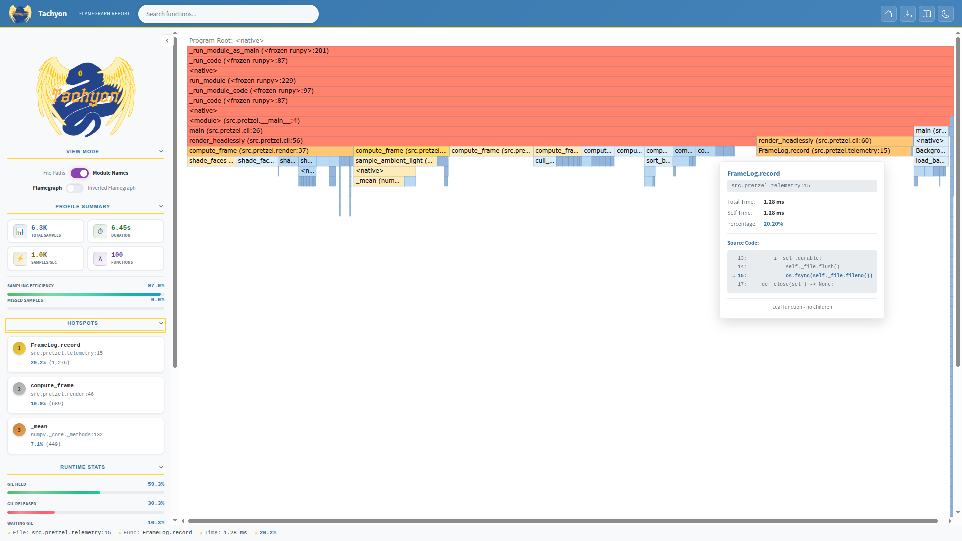
The report is a full-blown web application. You get a search box, a thread filter, zooming, an inverted view, and a sidebar that ranks the top hotspots next to gauges for sampling efficiency. Once again, FrameLog.record() leads at 20.2 percent. The <native> blocks sit right where Python crosses into NumPy and Tk.
Read a Line-Level Heatmap
Where flame graphs show structure, the heatmap report paints sample counts directly onto your source code:
$ uv run python -m profiling.sampling run --heatmap -o heatmap \
    -m pretzel --frames 300
Rendered 300 frames in 6.04s (49.7 fps)
Captured 6,467 samples in 6.47 seconds
Sample rate: 1,000.00 samples/sec
Error rate: 1.89
Heatmap output written to heatmap/
  - Index: heatmap/index.html
  - 43 source files analyzed
The command produces a directory named heatmap/ with an index.html ranking all source files. There are forty-three of them for this run, including the standard library and NumPy internals. There’s one page per file with a color gradient over the hot lines. For example, in shading.py, the NumPy lighting glows brightest:
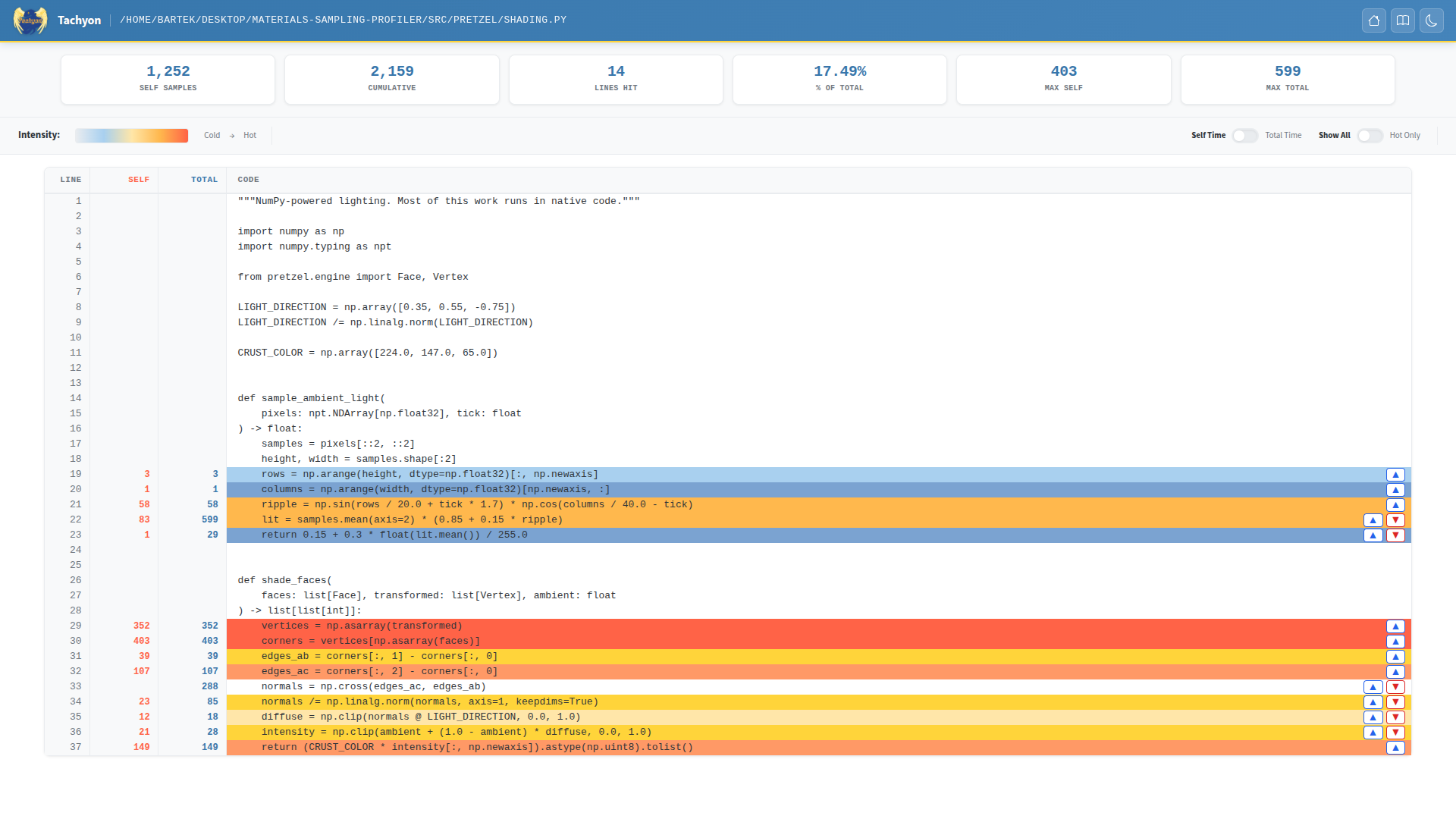
These hot lines are single expressions, yet the heatmap still picks them apart. Line 30’s fancy indexing burns the deepest red at 403 self samples, with the np.asarray(transformed) conversion on the line above running a close second. Flip the toggle at the top from Self Time to Total Time, and line 22’s samples.mean() reduction lights up instead at 599 cumulative samples.
When you already know the guilty function, the heatmap is the fastest way to find the guilty line.
Export to Firefox Profiler and Other Tools
Three more formats connect the sampler to an existing ecosystem of analysis tools:
--geckowrites the JSON format understood by Firefox Profiler, giving you a per-thread timeline that distinguishes Python code from native code and marks GIL waits.--collapsedemits classic folded stacks, one line per unique stack with a sample count, ready for Brendan Gregg’s originalflamegraph.plor any tool that eats that format.--jsonlstreams newline-delimited JSON with string, frame, and sample tables, including line and column spans for every frame, in case you want to build your own tooling on top.
Each of these accepts -o to pick the output path, just like the formats you’ve already used.
Record Binary Profiles and Replay Them Later
Every mode you’ve seen so far analyzes samples on the fly. Sometimes, you’d rather capture now and decide on the presentation later—for example, when you profile on a server but analyze the results from your laptop. The profiler supports that workflow with a compact binary format, a replay subcommand, and one especially useful combination of the two: differential flame graphs.
Capture Once, Convert Anytime
The --binary flag records raw samples to disk instead of aggregating them:
$ uv run python -m profiling.sampling run --binary -o slow.bin \
    -m pretzel --frames 300
Rendered 300 frames in 6.12s (49.0 fps)
Captured 6,541 samples in 6.54 seconds
Sample rate: 1,000.00 samples/sec
Error rate: 2.02
  Binary Encoding:
    Records:          5,011
      RLE repeat:     662 (13.2%) [2,060 samples]
      Full stack:     3 (0.1%)
      Suffix match:   19 (0.4%)
      Pop-push:       4,327 (86.4%)
  Frame Efficiency:
    Frames written:   7,147
    Frames saved:     75,600 (91.4%)
    Bytes (pre-zstd): 105.0 KB
Binary profile written to slow.bin (6409 samples)
The profiler encodes consecutive call stacks and, when available, compresses the result with Zstandard from the new compression.zstd module. Because it stores only the differences between stacks rather than each full stack, the profiler skips writing 91.4 percent of frames outright.
The replay subcommand then converts a recording into any of the other formats, defaulting to the pstats one, as if you were profiling live:
$ uv run python -m profiling.sampling replay slow.bin
Replaying 6409 samples from slow.bin
  Sample interval: 1000 us
  Compression: none
  [████████████████████████████████████████] 100.0% (6,409/6,409)
Profile Stats:
(...)
Notice that the output reports no compression. That’s because the uv-installed interpreters lack zstd support in the profiler’s writer, so compression falls back to none even though the compression.zstd module itself imports fine. Building CPython from source against libzstd-dev—which you can do with pyenv—compresses the capture instead.
You can render the same samples in other formats by choosing a different flag, for example:
$ uv run python -m profiling.sampling replay --flamegraph -o slow.html slow.bin
Replaying 6409 samples from slow.bin
  Sample interval: 1000 us
  Compression: none
  [████████████████████████████████████████] 100.0% (6,409/6,409)
Flamegraph data: 1 root function, 6409 total samples, 493 unique strings
Flamegraph saved to: slow.html
Replayed 6409 samples
Recording once and replaying later decouples when you capture a profile from how you analyze it. You can grab a binary snapshot in production, archive it, and revisit the same samples later in any format without rerunning your workload. That flexibility shines when you compare two profiles.
Next, you’ll capture a baseline, apply a fix, and let a differential flame graph reveal exactly what changed.
Prove Your Fix With a Differential Flame Graph
Recorded baselines unlock the neatest trick in the profiler’s repertoire. When you pass the captured samples to --diff-flamegraph, the profiler runs your program as usual, then renders the fresh samples against the baseline as a differential flame graph. It looks like a regular flame graph, but it overlays two runs in a single picture. Here’s how to interpret the visual cues:
- Widths show the current run, exactly like in the flame graph you generated earlier.
- Colors show the change against the baseline. A frame turns blue where a function’s own work shrank, red where it grew, gray where it held steady, and purple where the function is new and has no baseline to compare against. The more saturated the color, the bigger the shift.
There’s a twist that makes these graphs confusing at first. The colors track proportions, not wall-clock time. The profiler scales the baseline to the current run’s length before comparing, so when some work disappears, everything that remains claims a larger share of a smaller pie. On a successful diff, untouched code reddens a little—not because it got slower, but because it now matters more.
Start with the happy path by circling back to the hottest CPU line you found earlier. Line 46 of render.py builds a hexadecimal color string for every polygon on every frame. However, the shading pipeline derives all of those colors from a single brightness value, so the roughly 3,500 visible triangles share fewer than 300 distinct colors per frame. That makes the f-string a perfect candidate for memoization:
src/pretzel/render.py
# ...

_HEX_CACHE: dict[tuple[int, int, int], str] = {}

def hex_color(red: int, green: int, blue: int) -> str:
    key = (red, green, blue)
    color = _HEX_CACHE.get(key)
    if color is None:
        color = _HEX_CACHE[key] = f"#{red:02x}{green:02x}{blue:02x}"
    return color
Pretzel wires this cache to a --cache-colors flag, which routes the color formatting in compute_frame() through hex_color() instead of running the f-string every time. Crucially, the flag doesn’t rename or restructure anything. The same functions run in the same places—one of them just got cheaper.
Profile the optimized build against your recorded baseline now:
$ uv run python -m profiling.sampling run --diff-flamegraph slow.bin \
    -o diff-colors.html -m pretzel --frames 300 --cache-colors
Rendered 300 frames in 5.52s (54.3 fps)
Captured 5,951 samples in 5.95 seconds
Sample rate: 1,000.00 samples/sec
Error rate: 3.60
Flamegraph data: 1 root function, 5737 total samples, 525 unique strings
Flamegraph saved to: diff-colors.html
The result is the differential flame graph at its clearest:
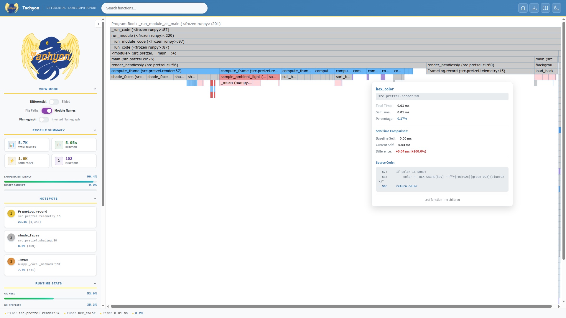
The wide compute_frame() band turns solid blue because its own share of the run fell by roughly a third. That’s the direct fingerprint of your fix, sitting exactly where you made it. The functions below shade light red or gray as their slices grow slightly in a faster run. And if you look closely, then you’ll spot a tiny purple newcomer tucked under compute_frame(). It’s hex_color() itself, which didn’t exist in the baseline.
This example demonstrates the fundamental rule of differential flame graphs. A frame can turn blue only if the same function survives into both runs. Optimize a function in place, and the diff rewards you with a blue block right where you worked. But what happens when a fix removes work instead of shrinking it?
Read the Red When a Fix Removes Work
Pretzel’s --fast flag flips two more of its planted bottlenecks into their optimized paths. It replaces the byte-at-a-time PPM decoder with a vectorized NumPy one and lets the telemetry writer buffer log entries in memory instead of flushing them to disk on every frame. Compare the --fast build against the same baseline:
$ uv run python -m profiling.sampling run --diff-flamegraph slow.bin \
    -o diff.html -m pretzel --frames 300 --fast
Rendered 300 frames in 3.94s (76.2 fps)
Captured 4,044 samples in 4.04 seconds
Sample rate: 1,000.00 samples/sec
Error rate: 2.27
Flamegraph data: 1 root function, 3952 total samples, 524 unique strings
Flamegraph saved to: diff.html
This time, the graph looks radically different:
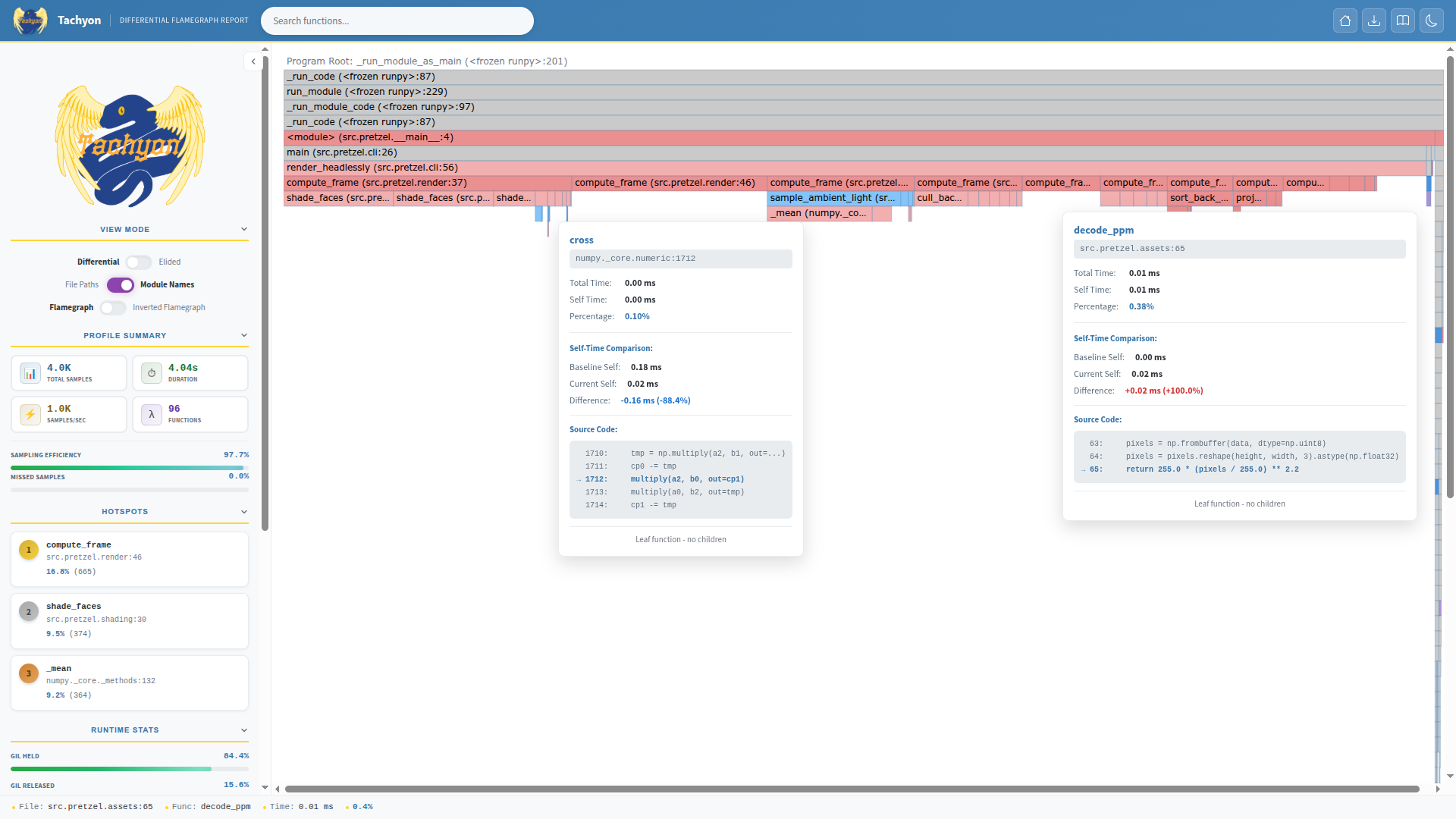
Don’t look for big blue blocks where the fixes went, because neither one can produce any:
- The old parser wasn’t optimized in place. It was replaced. To the profiler,
decode_ppm()is a brand-new function with no baseline to compare against, so it shows up purple, and barely a speck at that, because the vectorized decoder hardly registers in the samples. - The telemetry fix kept
FrameLog.record()in place, but a buffered write completes in microseconds. At a thousand snapshots per second, the sampler never catches the function in the act again, so it vanishes from the graph entirely, leaving nothing to color blue.
So where’s the evidence of your speedup? It’s the sea of red. The geometry and shading code that you didn’t touch—compute_frame(), shade_faces(), cull_backfaces()—could only balloon to a bigger share of the graph because the work around it collapsed. On a proportional chart, the red is the proof, and the header backs it up. The same three hundred frames now take about four seconds instead of six.
There’s one more subtlety hiding in the picture. The few blue frames that do appear sit in unexpected places, such as NumPy’s cross() in the shading code.
Remember from GIL mode that the wasteful parser was hogging the interpreter from its background thread. In the baseline, the renderer’s NumPy calls spent extra wall-clock time waiting for the lock, and that wait was billed to them. With the parser fixed, the contention is gone, and the old bottleneck’s victims cool down to blue. Your fix can show up not where you made it, but on the code that the bottleneck used to starve.
Note: Call stacks that appear only in the baseline, such as import-time work, are hidden from the main view. Use the Elided toggle in the report’s sidebar to reveal them.
Hover over any frame to see its exact before-and-after shares. For the record, the color cache alone lifts headless Pretzel from about 50 to 55 frames per second, while --fast pushes it past 75. Optimizing without measuring is guessing. But a differential flame graph turns each before-and-after comparison into a single picture that tells you what changed, what didn’t, and why.
Inspect a Live Python Process
Every command so far started the target program through the profiler. This last set of features works the other way around, and it’s what makes the new profiler a genuine observability tool rather than just a development aid. You’ll attach to a process that’s already running, watch its statistics update live, and drill all the way down to single bytecode instructions.
Attach to a Running Process
The attach subcommand takes the PID of any running Python 3.15 process—your web app misbehaving in production, say—and starts sampling without restarting, pausing, or instrumenting the target.
Note: Both the profiler and the profiled process must run the same version of Python. Otherwise, you might get the following error:
Can't attach from a pre-release Python interpreter
⮑ to a process running a different Python version
The versions must agree down to the minor part of the semantic version. For example, both processes must run Python 3.15, though the exact patch release, like 3.15.0 versus 3.15.1, doesn’t matter. Pre-releases are stricter, so 3.15.0b4 attaches only to 3.15.0b4.
Start the viewer with uv run pretzel and try attaching to it from another terminal:
$ uv run python -m profiling.sampling attach $(pgrep -n -f "pretzel$")

🔒 Tachyon was unable to access process memory. This could be because tachyon
has insufficient privileges (the required capability is CAP_SYS_PTRACE).
Unprivileged processes cannot trace processes that they cannot send signals
to or those running set-user-ID/set-group-ID programs, for security reasons.

If your uid matches the uid of the target process you want to analyze, you
can do one of the following to get 'ptrace' scope permissions:

* If you are running inside a Docker container, you need to make sure you
  start the container using the '--cap-add=SYS_PTRACE' or '--privileged'
  command line arguments. Notice that this may not be enough if you are not
  running as 'root' inside the Docker container as you may need to disable
  hardening (see next points).

* Try running again with elevated permissions by running 'sudo -E !!'.

* You can disable kernel hardening for the current session temporarily (until
  a reboot happens) by running 'echo 0 | sudo tee /proc/sys/kernel/yama/ptrace_scope'.
That cryptic message is a permission problem in disguise. Reading another process’s memory is a debugger-level privilege, so on most Linux distributions, the Yama security module lets a process trace only its own children by default. The run subcommand always works because the profiler is the parent of the process it spawns. To attach to an unrelated process, you need elevated privileges.
Rerun the command with sudo, just as you did earlier when profiling native code, and then stop the profiler with Ctrl+C after a few seconds. Alternatively, you can pass the --duration option to have the profiler automatically detach after the specified number of seconds, leaving the target undisturbed:
$ sudo .venv/bin/python -m profiling.sampling attach --duration 5 \
    --sort tottime -l 10 $(pgrep -n -f "pretzel$")
Captured 5,000 samples in 5.00 seconds
Sample rate: 1,000.00 samples/sec
Error rate: 9.76
Profile Stats:
       nsamples   sample%   tottime (s)    cumul%   cumtime (s)  filename:lineno(function)
      2411/2411      53.4         2.411      53.4         2.411  __init__.py:3075(Canvas._create)
        366/366       8.1         0.366       8.1         0.366  __init__.py:3077(Canvas._create)
        279/279       6.2         0.279       6.2         0.279  telemetry.py:15(FrameLog.record)
        201/201       4.5         0.201       4.5         0.201  __init__.py:3122(Canvas.delete)
       167/4512       3.7         0.167     100.0         4.512  __init__.py:1631(Misc.mainloop)
        139/139       3.1         0.139       3.1         0.139  render.py:46(compute_frame)
          87/87       1.9         0.087       1.9         0.087  shading.py:30(shade_faces)
          77/77       1.7         0.077       1.7         0.077  _methods.py:132(_mean)
          75/75       1.7         0.075       1.7         0.075  shading.py:29(shade_faces)
        68/2953       1.5         0.068      65.4         2.953  viewer.py:57(Viewer.render_next_frame)
(...)
Would you look at that! The windowed Pretzel viewer has an entirely different profile from the headless benchmark.
Over half the time goes into Canvas._create(), which is the Tkinter method that draws each polygon on screen. It’s code that the headless benchmark never ran at all. With a real window in the picture, redrawing thousands of polygons per frame costs more than computing them, pushing the hotspots you chased earlier, like FrameLog.record() and compute_frame(), far down the list.
A stripped-down benchmark can cover only the code it exercises, so profiles of your program in its real deployment can tell a very different story from benchmarks on your laptop. Attaching is how you get those profiles.
A few facts to keep in mind before you SSH into a production box:
- Permissions: On Linux, you need to run the profiler as
root, hold theCAP_SYS_PTRACEcapability, or relax theptrace_scopesetting. On macOS, you needsudo. On Windows, you need administrator rights orSeDebugPrivilege. - Version matching: The profiler and the target must run the same minor Python version, and pre-releases must match exactly. Attaching from your system’s Python 3.13 to a 3.15 process won’t work, which is why the command above invokes the interpreter inside the project’s
.venv/directory explicitly. - Security: Anything that can read another process’s memory can read its secrets, too. Treat profiling access accordingly.
Attaching gives you a rolling profile over time, but that’s not the only way to look inside a live process. The dump subcommand that you met earlier points at a running process’s PID with the same elevated access as attach but takes a single stack snapshot instead of a stream of samples. Think of that snapshot as the traceback you’d normally get only when a program crashes—except dump prints one on demand, while the process keeps running.
That makes dump particularly handy when a service hangs and you want to know what it’s stuck on right now, especially with --all-threads to see every thread at once.
Watch Live Statistics in Your Terminal
Batch reports are great for archaeology, but sometimes you want to watch the patient’s vitals in real time. The --live flag turns the profiler into an interactive, top-like terminal dashboard, and it works with both run and attach:
$ sudo .venv/bin/python -m profiling.sampling attach \
    --live $(pgrep -n -f "pretzel$")
The dashboard refreshes ten times per second with a running tally of samples:

The header alone is a mini-lecture on your program’s health. It includes the achieved sampling rate, the share of failed stack reads, and a live breakdown of GIL possession, exception state, and garbage collection across threads. Reading this header, you can tell that the viewer holds the GIL only 30 percent of the time because it mostly runs inside Tk’s native drawing code.
Press S to cycle the sort order, T to switch between threads, / to filter by function name, P to pause, and Q to quit—or H for the full list of shortcuts. If you’ve ever wished for htop, but for Python functions, this is it.
Zoom in on Single Bytecode Instructions
Here’s a party trick that no other Python profiler can perform. Pass --opcodes, and the sampler records which bytecode instruction each frame was executing at every snapshot. The dump subcommand gives you a taste of it, but this time with -a to capture the streamer thread, too:
$ sudo .venv/bin/python -m profiling.sampling dump \
    --blocking --opcodes -a $(pgrep -n -f "pretzel$")
Stack dump for PID 34756, thread 34757 (most recent call last):
  File ".../lib/python3.15/threading.py", line 1180, in Thread._bootstrap  opcode=CALL
    self._bootstrap_inner()
  File ".../lib/python3.15/threading.py", line 1218, in Thread._bootstrap_inner  opcode=CALL
    self._context.run(self.run)
  File "src/pretzel/streaming.py", line 30, in BackgroundStreamer.run
⮑  opcode=CALL_BUILTIN_O (CALL)
    time.sleep(self._interval)

Stack dump, thread 34756 (main thread, has GIL; most recent call last):
  File ".venv/bin/pretzel", line 10, in <module>  opcode=CALL
    sys.exit(main())
  File "src/pretzel/cli.py", line 24, in main  opcode=CALL
    show_window(mesh, streamer, frame_log, args.cache_colors)
  File "src/pretzel/cli.py", line 41, in show_window  opcode=CALL
    Viewer(mesh, streamer, frame_log, cache_colors).run()
  File "src/pretzel/viewer.py", line 44, in Viewer.run  opcode=CALL
    self.window.mainloop()
  File ".../lib/python3.15/tkinter/__init__.py", line 1631, in Misc.mainloop
⮑  opcode=CALL
    self.tk.mainloop(n)
  File ".../lib/python3.15/tkinter/__init__.py", line 2158, in CallWrapper.__call__
⮑  opcode=CALL_EX_PY (CALL_FUNCTION_EX)
    return self.func(*args)
  File ".../lib/python3.15/tkinter/__init__.py", line 880, in Misc.after.<locals>.callit
⮑  opcode=CALL_EX_NON_PY_GENERAL (CALL_FUNCTION_EX)
    func(*args, **kw)
  File "src/pretzel/viewer.py", line 52, in Viewer.render_next_frame
⮑  opcode=CALL_PY_EXACT_ARGS (CALL)
    polygons = compute_frame(
  File "src/pretzel/render.py", line 37, in compute_frame
⮑  opcode=CALL_PY_EXACT_ARGS (CALL)
    channels = shading.shade_faces(ordered, transformed, ambient)
  File "src/pretzel/shading.py", line 29, in shade_faces
⮑  opcode=CALL_BUILTIN_FAST_WITH_KEYWORDS (CALL)
    vertices = np.asarray(transformed)
Each frame now reports its current opcode, and there’s a subtle detail hiding in plain sight. CALL_BUILTIN_O isn’t a regular opcode but a specialized one, with its generic form shown in parentheses. You’re watching the adaptive specializing interpreter from Python 3.11 at work, live, in a running process.
Profiling with --opcodes feeds the same information into the other outputs. Flame-graph tooltips, expandable heatmap panels, and the live dashboard all break down which instructions dominate each hot line, whether specialized or not.
For everyday bottleneck hunting, you won’t need this level of detail. But when you’re chasing interpreter-level mysteries, such as why a seemingly innocent line resists specialization or how the JIT compiler in Python 3.15 treats your hottest loop, it’s a rare kind of microscope to have in the standard library.
Choose the Right Profiler for the Job
The new sampling profiler completes the lineup rather than replacing the older tools. Here’s how the built-in options stack up now:
| Tool | Overhead | Best For |
|---|---|---|
profiling.tracing |
High | Exact call counts in short, local runs |
profiling.sampling |
Near zero | Long-running apps, production, threads, async |
perf support |
Low | C-level symbols across Python and native code |
Keep the sampler’s statistical nature in mind when you read its reports. Percentages wobble a little between runs, very short runs yield few samples, and functions that blink in and out of existence may not register at all. When in doubt, profile for longer or raise the sampling rate with the -r option. The defaults are a sensible starting point.
Conclusion
Python 3.15 turns profiling from a specialized chore into something you can casually point at any Python process, local or remote, and get an answer in seconds. The new profiling package cleans up a decades-old corner of the standard library. Plus, its sampling profiler brings production-grade observability—flame graphs, heatmaps, async awareness, and a live dashboard included—to every Python installation with no third-party tools.
In this tutorial, you’ve learned that:
- Python 3.15 reorganizes the profilers into a
profilingpackage following PEP 799, deprecatingprofile, and keepingcProfileas an alias forprofiling.tracing. - The sampling profiler reads a target process’s memory from outside, so profiled code runs at essentially full speed.
- Modes dissect wall-clock time, CPU time, and GIL contention, while
--all-threadsand--async-awaremake threads and asyncio tasks first-class citizens. - The profiler renders results as
pstatstables, flame graphs, heatmaps, Firefox Profiler exports, and binary recordings you can replay and diff later. - Attaching to a live process requires debugger-level privileges and a matching Python version, and the live TUI turns the profiler into
htopfor Python code.
There’s more to explore that didn’t fit here:
--subprocessesfollows your worker processes.--mode exceptionsamples only code with an exception in flight.--realtime-statsprints the sampler’s own health stats while it runs.
The official profiling documentation covers them all, and Real Python’s Profiling in Python tutorial remains the best place to sharpen your general optimization workflow.
Now go find out what your own code has been doing behind your back!
Get Your Code: Click here to download the free sample code you’ll use to explore the sampling profiler in Python 3.15.
Frequently Asked Questions
Now that you have some experience with the sampling profiler in Python 3.15, you can use the questions and answers below to check your understanding and recap what you’ve learned.
It’s a statistical profiler in the standard library’s new profiling.sampling module, code-named Tachyon. It periodically snapshots a process’s call stack from the outside—a thousand times per second by default—so the target keeps running at its normal speed.
No. Only the pure-Python profile module is deprecated, with removal planned for Python 3.17. The cProfile module remains available as a backward-compatible alias for the relocated profiling.tracing module.
Yes. The attach subcommand samples any live Python 3.15 process by its process ID without restarting or instrumenting it. You need debugger-level privileges, such as sudo on Linux or macOS, and the profiler must run the same Python version as the target.
Both sample a target process from the outside, and py-spy pioneered this approach for Python. The standard-library profiler requires no installation, understands 3.15’s interpreter internals, including async task stacks and specialized bytecode instructions, and adds a live TUI plus flame-graph, heatmap, and Firefox Profiler outputs. However, py-spy supports attaching to a wider range of Python versions.
Yes. Pass -a to sample all threads instead of just the main one, and --async-aware to reconstruct asyncio task stacks, optionally with --async-mode all to include tasks suspended at await expressions. Named tasks appear under their names in the report.
Take the Quiz: Test your knowledge with our interactive “Python 3.15 Preview: Sampling Profiler” quiz. You’ll receive a score upon completion to help you track your learning progress:
Interactive Quiz
Python 3.15 Preview: Sampling ProfilerTest your understanding of Python 3.15's new sampling profiler, from CPU and GIL modes to flame graphs, heatmaps, and attaching to a live process.