Choosing between Docling and LlamaParse comes down to how you want to extract tables from a PDF in Python: on your own machine or in the cloud. Docling runs locally as an open-source library, while LlamaParse parses through an LLM-guided cloud pipeline. This tutorial builds the same table extractor twice to compare quality, setup, output formats, speed, and cost using a single sample PDF.
By the end of this tutorial, you’ll understand that:
- IBM’s Docling parses entirely on your own machine, needs no API key, and adds no per-document cost.
- LlamaIndex’s LlamaParse uploads every PDF to the cloud and parses it through tiers from
fasttoagentic_plus. - Docling exports straight to Markdown, JSON, HTML, and pandas DataFrames, while LlamaParse splits the work across a Parse path and an Extract path.
- Docling applies a fixed layout-detection stack, whereas LlamaParse interprets each page with an LLM.
- On a ten-page financial PDF, LlamaParse finished in about 30 seconds versus roughly 82 seconds for Docling on CPU.
Both parsers in this tutorial target the same sample_report.pdf, a table-heavy ten-page excerpt from an SEC 10-K filing, so you can compare their output directly.
You should be comfortable installing Python packages and running scripts from the terminal. Familiarity with files in Python helps, plus pandas DataFrames if you want DataFrame output.
You’ll also need the following before diving into this tutorial:
-
Python 3.10 or newer: Docling requires at least Python 3.10. Although LlamaParse also runs on 3.9, using the same minimum keeps both tools in a single environment. If you’re not sure which version you have, then run
python --versionin your terminal. If you need to install or upgrade, follow the steps in the guide on installing Python. -
LlamaCloud account (LlamaParse only): You’ll need this account to generate an API key. Never paste your API key directly into source code. Store it as the
LLAMA_CLOUD_API_KEYenvironment variable instead. The setup section below shows how to install the SDK and export the key for your operating system. -
Sample PDF: Keep
sample_report.pdfin your working directory. You can find it in the tutorial downloads if you want to follow along. -
Virtual environment: Create and activate one before installing any packages. If virtual environments are new to you, then Python Virtual Environments: A Primer will get you up to speed.
The exact commands depend on your operating system:
Don’t worry if you’ve never parsed a PDF programmatically. This tutorial walks you through installation from scratch, a first parse, and a side-by-side output comparison.
Get Your Code: Click here to download the free sample code that you’ll use to extract tables from a PDF with Docling and LlamaParse.
Take the Quiz: Test your knowledge with our interactive “Docling vs LlamaParse: How to Extract PDF Tables in Python” quiz. You’ll receive a score upon completion to help you track your learning progress:
Interactive Quiz
Docling vs LlamaParse: How to Extract PDF Tables in PythonTest your understanding of extracting PDF tables in Python with Docling and LlamaParse, and of when to parse locally instead of in the cloud.
Metrics Comparison: Docling vs LlamaParse
Use this table as an at-a-glance summary of packages, infrastructure requirements, and ballpark performance before the walkthroughs below:
| Metric | Docling | LlamaParse |
|---|---|---|
| Python package | docling |
llama-cloud (>=2.9.0) |
| Minimum Python version | 3.10 | 3.9 |
| Additional downloads on first run | Yes, layout and table models (~500–600 MB) | No, parsing runs in the cloud |
| Time to first parse (fresh install) | Slower, model download first | Faster, pip and API key only |
| API key required | No | Yes, LLAMA_CLOUD_API_KEY |
| Documents leave your machine | No | Yes, PDFs are uploaded for server-side parsing |
| Internet required at parse time | No, once models are cached | Yes |
| Marginal cost per document | $0 (local compute only) | Free tier of 10,000 credits per month, then paid tiers |
| Parse tiers | Not applicable (single local pipeline) | fast, cost_effective, agentic, agentic_plus (tutorial uses agentic) |
| Typical parse time (ten-page PDF, see Benchmarks) | ~10–20 s (text-heavy), ~60–90 s (table-heavy) on CPU | ~30 s over the network on the sample PDF (not tied to local CPU) |
| GPU support | Optional, speeds up layout analysis | Not applicable (server-side) |
| Primary maintainer | IBM Research (open source, MIT) | LlamaIndex (managed SaaS) |
| Best-known strength | Structured local pipelines, DataFrame export | Zero-infra setup, charts and unusual layouts |
Note: The llama-parse and llama-cloud-services packages were deprecated in May 2026. See also LlamaIndex’s announcement of the new llama-cloud SDKs and Parse API v2. All LlamaParse examples in this tutorial use llama-cloud>=2.9.0, which targets Parse API v2.
The next section turns this comparison into a practical recommendation.
Setup and Operational Model
For day-to-day work, the practical details matter most: how you install each tool, whether you need an API key, and where the parsing runs. Every example below uses the same sample_report.pdf from the tutorial downloads, so you can compare output directly.
Docling: Open-Source Parsing on Your Own Machine
Docling installs like any other Python library, but its default OCR engine, RapidOCR, prefers the onnxruntime backend, which a plain pip install docling doesn’t include:
(.venv) $ python -m pip install "docling==2.102.2"
(.venv) $ python -m pip install "onnxruntime>=1.7.0,<2.0.0"
These two packages give Docling its core converter and the OCR backend that this tutorial expects.
Note: Without onnxruntime, parsing still completes on Docling 2.102.2. Auto OCR skips the onnxruntime RapidOCR path, skips EasyOCR if it isn’t installed, then selects RapidOCR with the torch backend that already ships with Docling. At the info level, you see lines like:
rapidocr cannot be used because onnxruntime is not installed.
easyocr cannot be used because it is not installed.
Auto OCR model selected rapidocr with torch.
That torch fallthrough isn’t the path this tutorial targets, so install onnxruntime as shown above.
Note: The pip install pulls in only the Python packages, on the order of tens of megabytes. The first time you parse a PDF, Docling downloads additional model weights over the network:
- Layout analysis (
docling-project/docling-layout-heron): Finds headings, tables, figures, and reading order. - Table structure (
docling-project/docling-models): Reconstructs rows and columns inside detected tables. - OCR (RapidOCR PP-OCRv6 ONNX weights): Loaded because OCR is enabled by default, even though those weights do little work on a PDF that already has embedded text.
Expect all this to take up roughly 500–600 MB on disk. Layout and table weights are cached by Hugging Face under ~/.cache/huggingface/hub/, or under $HF_HOME if you set that variable. RapidOCR stores its ONNX files inside your virtual environment at site-packages/rapidocr/models/.
To download everything ahead of your first parse, run docling-tools models download, which saves the models in ~/.cache/docling/models/ by default.
To reclaim the space later, uninstall the packages with pip uninstall docling onnxruntime, delete the Hugging Face cache folders whose names start with models--docling-project--, and remove ~/.cache/docling if you pre-downloaded models there. Deleting the virtual environment also removes the RapidOCR files.
After models are cached, parsing runs entirely on your machine. No API key, no outbound document upload, and no per-page billing.
The script below converts a local PDF to a structured DoclingDocument object, then exports it to Markdown:
docling_extraction.py
from pathlib import Path
from docling.document_converter import DocumentConverter

PDF_PATH = Path("sample_report.pdf")

def main() -> None:
    converter = DocumentConverter()
    result = converter.convert(PDF_PATH)

    markdown = result.document.export_to_markdown()
    print(markdown[:3000])
    print("\n---\n")
    print(f"Pages parsed: {len(result.document.pages)}")
    print(f"Tables found: {len(result.document.tables)}")

if __name__ == "__main__":
    main()
The DocumentConverter class is Docling’s entry point. It loads the default PDF pipeline, which covers layout analysis, OCR, and table structure. Calling .convert() with a file path runs that pipeline and returns a result object whose .document attribute is a structured DoclingDocument.
From there, .export_to_markdown() turns the parsed content into a Markdown string. The .pages and .tables attributes let you inspect what Docling found without reparsing.
Run the script from your project directory:
(.venv) $ python docling_extraction.py
On a laptop without a GPU, a ten-page text-heavy PDF commonly takes on the order of 10–20 seconds. Table-heavy financial pages take longer: this tutorial’s sample_report.pdf run took around 82 seconds on CPU (see Benchmarks). Attach a CUDA-capable GPU, and parsing often finishes in a few seconds.
Docling prints pipe-style Markdown tables for the financial index and operations statement, then reports page and table counts. The script shows only the first 3,000 characters of the Markdown output, and the individual lines below are shortened further to fit:
## Item 8. Financial Statements and Supplementary Data

| Index to Consolidated Financial Statements ... |   Page |
|------------------------------------------- ... |--------|
| Consolidated Statements of Operations ... |     29 |
| Consolidated Statements of Comprehensive ... |     30 |
| Consolidated Balance Sheets ... |     31 |
| Consolidated Statements of Shareholders' ... |     32 |
| Consolidated Statements of Cash Flows ... |     33 |
| Notes to Consolidated Financial ... |     34 |
| Reports of Independent Registered ... |     49 |

All financial statement schedules have been omitted,
since the required information is not applicable or is
not present in amounts sufficient  to  require  submission
of  the  schedule,  or  because  the  information  required
is  included  in  the  consolidated  financial statements
and accompanying notes.

## CONSOLIDATED STATEMENTS OF OPERATIONS

(In millions, except number of shares,
which are reflected in thousands, and
per-share amounts)

| | Years ended        | Years ended        | Years ended        |
| | Sep 27, 2025       | Sep 28, 2024       | Sep 30, 2023       |
| Net sales:           |                    |                    |
| Products             | $ 307,003          | $ 294,866          | ...
| Services             | 109,158            | 96,169             | ...
| Total net sales      | 416,161            | 391,035            | ...
| Cost of sales:       |                    |                    |
| Products             | 194,116            | 185,233            | ...
| Services             | 26,844             | 25,119             | ...
| Total cost of sales  | 220,960            | 210,352            | ...

---

Pages parsed: 10
Tables found: 10
You take on local model management in exchange for zero marginal cost and full data custody.
Docling fits teams that handle sensitive PDFs—HR records, contracts, and medical forms—or that need offline parsing in air-gapped environments.
LlamaParse: Managed API, Zero Model Management
LlamaParse moved to the unified llama-cloud SDK in May 2026. With your virtual environment active, install the package:
(.venv) $ python -m pip install "llama-cloud>=2.9.0"
Create an API key in the LlamaCloud dashboard. The free tier includes 10,000 credits per month, enough to prototype on dozens of documents. Store the key as an environment variable so it never touches your source code or version control history. Replace your-api-key-here with your actual API key, keeping the quotes around the string:
Note: Parse API v2 organizes parsing into tiers that trade speed, cost, and accuracy: fast, cost_effective, agentic, and agentic_plus. This tutorial uses agentic, LlamaIndex’s default recommendation for PDFs with tables and complex layouts. Older LlamaIndex blog posts refer to similar capabilities as Premium parsing modes. See the tiers guide for current names and credit costs.
Parsing runs in LlamaIndex’s cloud rather than on your own machine. The script below uploads sample_report.pdf, parses it with the agentic tier, and prints the first part of the Markdown response:
llamaparse_extraction.py
import os
from pathlib import Path
from llama_cloud import LlamaCloud

PDF_PATH = Path("sample_report.pdf")

def main() -> None:
    client = LlamaCloud(api_key=os.environ["LLAMA_CLOUD_API_KEY"])

    uploaded = client.files.create(file=PDF_PATH, purpose="parse")
    result = client.parsing.parse(
        file_id=uploaded.id,
        tier="agentic",
        version="latest",
        expand=["markdown"],
    )

    pages = ""
    for page in result.markdown.pages:
        pages += page.markdown
        pages += "\n---\n"

    print(pages[:3000])
    print(f"Pages parsed: {len(result.markdown.pages)}")

if __name__ == "__main__":
    main()
The flow is upload, then parse. The LlamaCloud() constructor creates an authenticated client using your API key. The files.create() method uploads the PDF to LlamaCloud and returns a file ID. The parsing.parse() method sends that ID to the Parse API with the agentic processing tier, sets version to latest, and asks for Markdown via expand=["markdown"].
The result’s markdown.pages list holds one Markdown string per page, which the loop stitches together before printing. Run the script from your project directory:
(.venv) $ python llamaparse_extraction.py
...
Pages parsed: 10
Because compute happens remotely, parse time stays consistent whether you’re on a developer laptop or a CI runner with minimal CPU.
LlamaParse returns the same financial content, but tables appear as HTML blocks inside the Markdown field rather than Docling’s pipe-style tables. Again, only the first 3,000 characters are shown, truncated for readability:
# Item 8. Financial Statements and Supplementary Data

<table>
  <thead>
    <tr>
      <th>Index to Consolidated Financial Statements</th>
      <th>Page</th>
    </tr>
  </thead>
  <tbody>
    <tr>
      <td><u>Consolidated Statements of Operations ...</u></td>
      <td>29</td>
    </tr>
    <tr>
      <td><u>Consolidated Balance Sheets ...</u></td>
      <td>31</td>
    </tr>
    ...
  </tbody>
</table>
---
# Apple Inc.

## CONSOLIDATED STATEMENTS OF OPERATIONS

<table>
  ...
  <tr>
    <td>Products</td>
    <td>307,003</td>
    <td>294,866</td>
    <td>298,085</td>
  </tr>
  <tr>
    <td>Total net sales</td>
    <td>416,161</td>
    <td>391,035</td>
    <td>383,285</td>
  </tr>
  ...
</table>

Pages parsed: 10
Every document passes through LlamaIndex’s servers. For confidential or regulated data, review LlamaIndex’s data-processing terms.
Note: If you’re already building on LlamaIndex, LlamaParse slots into ingestion pipelines with minimal glue code. Docling has its own LlamaIndex integration, but the default path is local conversion followed by framework-specific chunking.
Setup Summary
How you run a parser matters as much as how well it parses. The metrics comparison table above records the objective differences: packages, upload behavior, cost, and connectivity. The walkthroughs above show what those facts mean for sample_report.pdf.
For regulated or confidential PDFs, Docling is the stronger default: files stay on your machine. LlamaParse trades that custody for managed infrastructure. You skip the local model download, but your files leave your network.
Which of those facts actually decides the question depends on the constraints you’re working under. In the tool below, select the ones that apply to you and each parser resolves to viable, viable with a caveat, or ruled out, with the reason named. The dashed rule between the two panels is the trust boundary: watch what happens to it when you rule the cloud option in or out.
Extract Tables From a PDF in Python
Both Docling and LlamaParse aim to preserve reading order, recover tables, and handle non-trivial layouts. They reach those goals through different architectures, and the difference shows up in the output.
Docling: Layout Analysis and Table Structure
Docling runs a fixed layout-detection stack on every page. A layout model labels headings, tables, figures, and paragraphs as distinct regions, and a table-structure model rebuilds rows and columns inside those table regions. Pipeline rules then assemble the reading order from those labeled boxes. The same models and rules apply to every document, so nothing reinterprets the page at runtime.
For digital-born PDFs with embedded text, Docling reads the text layer directly rather than running full-page OCR, so you avoid recognition errors on clean documents and save processing time. OCR still runs on bitmap regions when needed, and Docling falls back to it automatically on scanned PDFs.
The setup run above shows what Docling produced on this ten-page SEC filing excerpt: ten detected tables rendered as pipe-style Markdown, plus section headings such as ## Item 8. Financial Statements and Supplementary Data. Treat that as one observed run on a bordered-table financial report, not a guarantee for every annual report or technical manual.
Docling’s documented and community-reported limitations include:
- Borderless tables: Tables defined only by whitespace can be misread, merged incorrectly, or detected as both a table and a figure. See
do_cell_matchingin the Docling pipeline options and GitHub issue #3495. - Dense multi-column layouts: Reading order can follow PDF object order rather than column-first flow on research-paper layouts. See GitHub discussion #2791 and issue #2201.
For table-heavy workflows, Docling attaches each detected table to the parsed DoclingDocument. The script below lists every table’s page provenance and DataFrame shape, then exports the financial index and operations statement from sample_report.pdf:
docling_tables.py
from pathlib import Path
from docling.document_converter import DocumentConverter

PDF_PATH = Path("sample_report.pdf")

def main() -> None:
    document = DocumentConverter().convert(PDF_PATH).document

    print(f"Tables found: {len(document.tables)}\n")

    for index, table in enumerate(document.tables):
        pages = sorted({prov.page_no for prov in table.prov})
        frame = table.export_to_dataframe(doc=document)
        print(f"Table {index}: pages {pages}, shape {frame.shape}")

    index_table = document.tables[0].export_to_dataframe(
        doc=document
    )
    print("\nFinancial statement index (table 0):")
    print(index_table.to_string(index=False), end="\n\n")

    operations_table = document.tables[1].export_to_dataframe(
        doc=document
    )
    print("Operations statement preview (table 1, first 4 rows):")
    print(operations_table.head(4).to_string())

if __name__ == "__main__":
    main()
The list document.tables holds the detected tables. Each table.prov entry records where that table appeared in the source PDF, and page_no is 1-based. The method .export_to_dataframe(doc=document) turns a single table into a pandas DataFrame without reparsing the file.
Run it and see what Docling found:
(.venv) $ python docling_tables.py
On sample_report.pdf, Docling finds ten tables: one per major financial statement page, plus segment and fair-value disclosures later in the excerpt:
Tables found: 10

Table 0: pages [1], shape (7, 2)
Table 1: pages [2], shape (24, 4)
Table 2: pages [3], shape (13, 4)
Table 3: pages [4], shape (35, 3)
Table 4: pages [5], shape (19, 4)
Table 5: pages [6], shape (34, 4)
Table 6: pages [9], shape (7, 4)
Table 7: pages [9], shape (8, 4)
Table 8: pages [10], shape (16, 8)
Table 9: pages [10], shape (16, 8)

Financial statement index (table 0):
Consolidated Statements of Operations for the years
    ended September 27, 2025, September 28, 2024 and September 30, 2023   29
Consolidated Statements of Comprehensive Income for the years
    ended September 27, 2025, September 28, 2024 and September 30, 2023   30
Consolidated Balance Sheets as of
    September 27, 2025 and September 28, 2024   31
Consolidated Statements of Shareholders' Equity for the years
    ended September 27, 2025, September 28, 2024 and September 30, 2023   32
Consolidated Statements of Cash Flows for the years ended
    September 27, 2025, September 28, 2024 and September 30, 2023   33

Notes to Consolidated Financial Statements   34
Reports of Independent Registered Public Accounting Firm   49

Operations statement preview (table 1, first 4 rows):
                   Years ended.September 27, 2025
                   Years ended.September 28, 2024
                   Years ended.September 30, 2023
0       Net sales:
1    Products            $ 307,003     $ 294,866     $ 298,085
2    Services                109,158          96,169           85,200
3   Total net sales       416,161          391,035        383,285
On this sample, each table maps to a single page. For tables that span multiple pages, check table.prov for more than one page entry and verify that row headers repeat correctly before loading the DataFrame into downstream analytics.
On scanned PDFs, Docling’s OCR path is slower but usually faithful on printed text. Expect more cleanup on low-resolution scans or documents with heavy watermarking.
LlamaParse: LLM-Guided Page Interpretation
Where Docling applies the same layout-detection stack to every page, LlamaParse’s agentic tier takes a different path: it sends each page to an LLM-guided parser in the cloud. Instead of classifying regions with specialized layout models, the LLM interprets visual structure from the page itself. That difference shows up on documents where Docling’s rule-based detectors struggle:
- Tables missed by rule-based detection: Regions that Docling’s layout model never labels as tables.
- Charts and figures: Diagrams that the parser describes in natural language for downstream LLMs.
- Unusual templates: Documents that don’t match the layouts Docling’s models were trained on.
That flexibility comes with its own failure mode. In two-column research PDFs, parsers can interleave text across columns by reading one line from the left column, then one from the right, rather than finishing each column first.
LlamaIndex describes this as a core multi-column parsing challenge in its glossary and has noted column mixing across parse modes.
LlamaIndex’s v1-to-v2 migration guide replaces parse_mode with tier and drops premium_mode entirely, and its Premium mode comparison covers that older naming in more detail.
Users parsing complex layouts have attempted to correct column order with custom prompts (agentic_options.custom_prompt in Parse API v2), with mixed results. See GitHub issue #229 for one open report where explicit column-reading instructions were not followed. The sample_report.pdf examples here are single-column financial pages, so you won’t see this failure mode.
For table-heavy workflows on the same PDF, LlamaParse’s Parse path doesn’t expose a document.tables list. Tables arrive as HTML <table> blocks inside each page’s Markdown. The script below reuses the upload-and-parse flow from setup, finds those blocks, and prints the financial index and operations statement:
llamaparse_tables.py
import os
import re
from pathlib import Path
from llama_cloud import LlamaCloud

PDF_PATH = Path("sample_report.pdf")
TABLE_PATTERN = re.compile(
    r"<table\b.*?</table>", re.DOTALL | re.IGNORECASE
)

def main() -> None:
    client = LlamaCloud(api_key=os.environ["LLAMA_CLOUD_API_KEY"])

    uploaded = client.files.create(file=PDF_PATH, purpose="parse")
    result = client.parsing.parse(
        file_id=uploaded.id,
        tier="agentic",
        version="latest",
        expand=["markdown"],
    )

    tables = []
    for page_no, page in enumerate(result.markdown.pages, start=1):
        for table_html in TABLE_PATTERN.findall(page.markdown):
            tables.append((page_no, table_html))

    print(f"Tables found: {len(tables)}\n")
    for index, (page_no, table_html) in enumerate(tables):
        print(f"Table {index}: page {page_no}")

    print("\nTable 0:")
    print(tables[0][1], end="\n\n")

    print("Table 1 (truncated):")
    print(tables[1][1][:700], "...")

if __name__ == "__main__":
    main()
Each match is one HTML table string plus the 1-based page it came from. That’s the LlamaParse equivalent of Docling’s table.prov and document.tables loop: page provenance is still there, but you scrape it out of Markdown instead of reading a typed table object.
You can execute this script the same way:
(.venv) $ python llamaparse_tables.py
On sample_report.pdf, LlamaParse finds the same ten tables, and they arrive as HTML rather than pipe-style Markdown. The listing below is truncated for display:
Tables found: 10

Table 0: page 1
Table 1: page 2
Table 2: page 3
Table 3: page 4
Table 4: page 5
Table 5: page 6
Table 6: page 9
Table 7: page 9
Table 8: page 10
Table 9: page 10

Table 0:
<table>
  <thead>
    <tr>
      <th>Index to Consolidated Financial Statements</th>
      <th>Page</th>
    </tr>
  </thead>
  <tbody>
    <tr>
      <td><u>Consolidated Statements of Operations ...</u></td>
      <td>29</td>
    </tr>
    <tr>
      <td><u>Consolidated Balance Sheets ...</u></td>
      <td>31</td>
    </tr>
    ...
  </tbody>
</table>

Table 1 (truncated):
<table>
  <thead>
    <tr>
      <th></th>
      <th></th>
      <th>Years ended</th>
      <th></th>
    </tr>
    <tr>
      <th></th>
      <th>September 27,</th>
      <th>September 28,</th>
      <th>September 30,</th>
    </tr>
    <tr>
      <th></th>
      <th>2025</th>
      <th>2024</th>
      <th>2023</th>
    </tr>
  </thead>
  <tbody>
    <tr>
      <td>Net sales:</td>
      <td></td>
      <td></td>
      <td></td>
    </tr>
    <tr>
      <td>Products</td>
      <td>307,003</td>
      <td>294,866</td>
      <td>298,085</td>
    </tr>
    <tr>
      <td>Services</td>
      <td>109,158</td>
      <td>96,169</td>
      <td>85,200</td>
    </tr>
    <tr>
      <td>Total net sales</td>
      <td>416,161</td>
      <td>391,035</td>
      <td>383,285</td>
    </tr>
    ...
  </tbody>
</table>
When LlamaParse describes a chart or diagram, that description is natural language meant for LLM consumption, not a machine-readable data series. If you need numeric values from a plot, then plan on a dedicated chart-extraction step regardless of which parser you choose.
Output Formats
With the setup scripts above in place, each parser exports the same sample_report.pdf differently. The right output format depends on whether you’re building RAG, analytics, or human-readable previews. Docling and LlamaParse differ meaningfully here, from Markdown and JSON to direct pandas DataFrames and schema-driven extraction.
Docling: Markdown, JSON, HTML, and DataFrames
The script below writes Markdown, JSON, and HTML files from one parsed DoclingDocument and prints DataFrame previews for each table:
docling_formats.py
import json
from pathlib import Path
from docling.document_converter import DocumentConverter

PDF_PATH = Path("sample_report.pdf")

def main() -> None:
    converter = DocumentConverter()
    document = converter.convert(PDF_PATH).document

    markdown = document.export_to_markdown()
    Path("output_docling.md").write_text(
        markdown, encoding="utf-8"
    )

    payload = document.export_to_dict()
    Path("output_docling.json").write_text(
        json.dumps(payload, indent=2),
        encoding="utf-8",
    )

    html = document.export_to_html()
    Path("output_docling.html").write_text(
        html, encoding="utf-8"
    )

    for index, table in enumerate(document.tables):
        frame = table.export_to_dataframe(doc=document)
        print(f"Table {index} shape: {frame.shape}")
        print(frame.head(), end="\n\n")

if __name__ == "__main__":
    main()
The standout integration feature is table.export_to_dataframe(). If your pipeline ends in pandas, Polars, or a SQL loader, then you can skip a separate table-scraping step entirely. The script loops over all ten tables and prints .head() for each, but the truncated output below shows only the first two:
Table 0 shape: (7, 2)
          Index to Consolidated Financial Statements
          Page
0  Consolidated Statements of Operations for the ...   29
1  Consolidated Statements of Comprehensive Incom...   30
2  Consolidated Balance Sheets as of September 27...   31
3  Consolidated Statements of Shareholders' Equit...   32
4  Consolidated Statements of Cash Flows for the ...   33

Table 1 shape: (24, 4)
                    ... Years ended.September 30, 2023
0       Net sales:  ...
1         Products  ...                      $ 298,085
2         Services  ...                         85,200
3  Total net sales  ...                        383,285
4   Cost of sales:  ...

[5 rows x 4 columns]
...
The JSON export preserves the full DoclingDocument tree, including metadata and cross-references to texts and tables. The excerpt below comes from output_docling.json:
{
  "schema_name": "DoclingDocument",
  "version": "1.10.0",
  "name": "sample_report",
  "origin": {
    "mimetype": "application/pdf",
    "filename": "sample_report.pdf"
  },
  "body": {
    "children": [
      { "$ref": "#/texts/0" },
      { "$ref": "#/tables/0" },
      { "$ref": "#/texts/1" }
    ]
  }
}
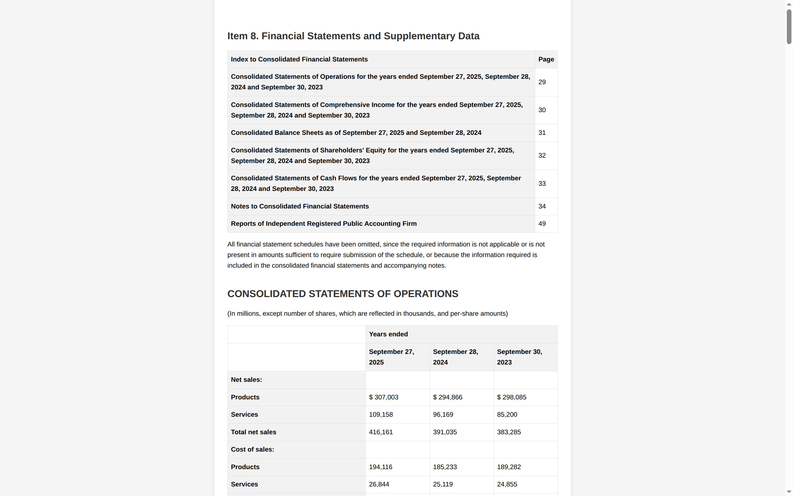
The HTML export renders headings and tables. The screenshot below shows output_docling.html in a browser:
LlamaParse: Markdown, Text, and Schema-Driven JSON
The llama-cloud SDK exposes two complementary paths for getting data out of a PDF:
- Parse path (
client.parsing.parse()) recovers narrative content: headings, paragraphs, and tables. Passexpand=["markdown", "text"]to request page-by-page Markdown and plain text for RAG pipelines or human preview. Parse API v2 doesn’t offer a standalone HTML export. Table structure arrives as HTML blocks inside the Markdown field. - Extract path (
client.extract.run()) returns typed fields. You supply a JSON Schema from your Pydantic model inconfiguration["data_schema"], setextraction_targetto control granularity, and the API responds with validated JSON you can load directly into Python objects or a database.
The script below uploads sample_report.pdf twice—once for the Parse path and once for the Extract path—and writes Markdown, text, and JSON files:
llamaparse_formats.py
import json
import os
from pathlib import Path
from llama_cloud import LlamaCloud
from pydantic import BaseModel, Field

PDF_PATH = Path("sample_report.pdf")

class RevenueRow(BaseModel):
    period: str = Field(
        description="Fiscal period label, e.g. FY 2025 or September 27, 2025",
    )
    revenue_millions: float = Field(
        description="Revenue in millions of USD",
    )
    growth_percent: float | None = Field(
        default=None,
        description="Year-over-year growth percentage if stated",
    )

class RevenueTable(BaseModel):
    rows: list[RevenueRow] = Field(
        description="One row per fiscal period in the table"
    )

def main() -> None:
    client = LlamaCloud(api_key=os.environ["LLAMA_CLOUD_API_KEY"])

    uploaded = client.files.create(file=PDF_PATH, purpose="parse")

    parsed = client.parsing.parse(
        file_id=uploaded.id,
        tier="agentic",
        version="latest",
        expand=["markdown", "text"],
    )

    markdown_pages = "\n\n".join(
        page.markdown for page in parsed.markdown.pages
    )
    Path("output_llamaparse.md").write_text(
        markdown_pages, encoding="utf-8"
    )

    if parsed.text and parsed.text.pages:
        text_pages = "\n".join(
            page.text for page in parsed.text.pages
        )
        Path("output_llamaparse.text").write_text(
            text_pages, encoding="utf-8"
        )

    extract_file = client.files.create(
        file=PDF_PATH, purpose="extract"
    )
    job = client.extract.run(
        file_input=extract_file.id,
        configuration={
            "data_schema": RevenueTable.model_json_schema(),
            "extraction_target": "per_doc",
            "tier": "agentic",
        },
    )

    Path("output_llamaparse.json").write_text(
        json.dumps(job.extract_result, indent=2),
        encoding="utf-8",
    )
    print(json.dumps(job.extract_result, indent=2))

if __name__ == "__main__":
    main()
The first half of main() runs the Parse path: it uploads the file with .create(), then calls .parse() and saves the Markdown and plain-text outputs. The second half runs the Extract path: it uploads the PDF again, then calls .run() with a JSON Schema built from RevenueTable to produce output_llamaparse.json.
Jobs on the Extract path run asynchronously in LlamaCloud. The client.extract.create() method submits the job and returns immediately with a job ID, while the server keeps processing in the background. You then call .get(job_id) in a loop or use .wait_for_completion(job_id) until the status becomes COMPLETED. That repeated status check is polling.
The .run() method wraps those steps in one call. It invokes .create(), polls until the job finishes, and returns the completed result. The official SDK examples often show the longer form explicitly, but both approaches return the same structured output.
The Parse path writes output_llamaparse.md, where the tables keep the same HTML shape you saw for the financial index and operations statement in Extract Tables From a PDF in Python. A representative excerpt from that file appears below:
# Item 8. Financial Statements and Supplementary Data

<table>
  <thead>
    <tr>
      <th>Index to Consolidated Financial Statements</th>
      <th>Page</th>
    </tr>
  </thead>
  <tbody>
    <tr>
      <td><u>Consolidated Statements of Operations ...</u></td>
      <td>29</td>
    </tr>
    <tr>
      <td><u>Consolidated Balance Sheets ...</u></td>
      <td>31</td>
    </tr>
    ...
  </tbody>
</table>
The plain-text output is saved to output_llamaparse.text. It keeps the same reading order as the Markdown output, but it isn’t fully plain: inline tags such as <u> can survive into the text output:
Item 8.   Financial Statements and Supplementary Data

 Index to Consolidated Financial Statements
 Page
 <u>Consolidated Statements of Operations for the years
 ended September 27, 2025 ...</u>                         29
 <u>Consolidated Balance Sheets as of September 27, 2025
 and September 28, 2024</u>                              31
 ...
The Extract path writes output_llamaparse.json, validated JSON matching the Pydantic schema:
{
  "rows": [
    {
      "period": "2025",
      "revenue_millions": 209586.0,
      "growth_percent": null
    },
    {
      "period": "2024",
      "revenue_millions": 201183.0,
      "growth_percent": null
    },
    {
      "period": "2023",
      "revenue_millions": 200583.0,
      "growth_percent": null
    }
  ]
}
On this run, the model latched onto the iPhone segment row from page 9 ($209,586, $201,183, $200,583) rather than total net sales ($416,161, $391,035, $383,285), which both parsers recovered earlier in this tutorial. The schema constrained the shape, but the generic “Revenue in millions of USD” description was not specific enough to steer the Extract path to the operations statement.
That is the real lesson here: schema-driven extraction is only as good as your field descriptions.
The extraction_target: "per_doc" setting returns one JSON object for the whole document, which matches a single-table schema like RevenueTable.
Integration Comparison
When you’re ready to wire a parser into your pipeline, use this API chooser. It maps output goals to the right method:
| Need | Docling | LlamaParse |
|---|---|---|
| Markdown for RAG | .export_to_markdown() |
.parse() |
| DataFrame per table | .export_to_dataframe() |
.run() + row schema |
| Schema-driven fields | Post-process manually | .run() + Pydantic |
| LlamaIndex ingestion | Via extensions | Native integration |
Docling gives you direct, code-level access to a parsed document object, while LlamaParse splits the work across the Parse path and the Extract path.
Benchmarks: Timing the Same PDF
The setup scripts above both target sample_report.pdf. The tables below record one reproducible run of each Python parser on that PDF. The metrics comparison table summarizes those timings. Numbers vary by hardware, network, and PDF complexity, so don’t treat them as universal. Run your own timing on documents that match your real workload.
Still, that one run is enough to anchor the operational-model discussion with concrete numbers. Both scripts had run once already, so Docling parsed with its models cached:
(.venv) $ time python docling_extraction.py
...
real    1m22.378s
user    2m12.188s
sys     0m17.921s

(.venv) $ time python llamaparse_extraction.py
...
real    0m29.808s
user    0m0.560s
sys     0m0.091s
Note: The format of time output depends on your shell and operating system, so yours may look different.
The table below shows wall-clock time on the same ten-page, table-heavy financial report:
| Metric | Docling (CPU) | LlamaParse (cloud) |
|---|---|---|
Wall-clock time on sample_report.pdf |
82.4 s | 29.8 s |
On the same sample PDF, both parsers recovered the index and operations tables:
| Aspect | Docling | LlamaParse |
|---|---|---|
| Table structure | Both tables correct | Both tables correct |
| Export format | Pipe-style Markdown tables | HTML <table> blocks inside the Markdown field |
| Header handling | Operations header repeats Years ended in each column | Nested year headers via stacked <th> rows; other tables also use colspan |
The export shapes differ: Docling returns formatted Markdown, while LlamaParse returns HTML tables.
Note: Docling’s first run includes model download time for its layout and table-recognition models, which can add significant overhead. For a fair comparison, either pre-warm Docling with one throwaway run before timing or report first-run and steady-state numbers separately.
Conclusion
Docling and LlamaParse both extract tables from a PDF in Python, and they diverge on the axes that usually decide the winner: where parsing runs, what you pay per document, and what shape the output takes.
- Choose Docling if your documents are sensitive, you want no ongoing API cost, you need DataFrame or lossless JSON output, or you’re working offline. The local model stack requires more setup and hardware, but you keep full custody of your files.
- Choose LlamaParse if you want zero infrastructure to manage, your documents contain images or charts that benefit from LLM interpretation, you’re already on LlamaIndex, or consistent cloud-side speed matters more to you than keeping parsing local.
You don’t need to commit to one forever. Many teams prototype with LlamaParse for speed, then move stable, high-volume, or confidential workloads to Docling once the pipeline is settled. A hybrid approach is valid too—LlamaParse for messy one-off documents, Docling for the bulk of predictable corporate PDFs in a scheduled ETL job.
If your organization already blocks outbound uploads, the decision is largely made: running Docling locally is the practical default. If you’ve standardized on LlamaIndex for RAG, LlamaParse reduces integration friction, even when Docling’s Markdown output would otherwise fit the pipeline better.
Next Steps
Everything above rests on a single ten-page financial report, and your own documents will look different. Replace sample_report.pdf with one of your own PDFs and rerun the setup scripts. The trade-offs only become concrete once you compare each parser’s output on your tables and layouts.
If you’re piping parsed text into a RAG pipeline, Real Python’s guide to LlamaIndex in Python shows you how to load documents, build a persistent index, and query it for grounded answers. The companion video course on using LlamaIndex for RAG walks through the same workflow on screen.
For more on what happens after parsing, Real Python’s LLM Application Development With Python learning path covers prompting, retrieval pipelines, and agents.
Get Your Code: Click here to download the free sample code that you’ll use to extract tables from a PDF with Docling and LlamaParse.
Frequently Asked Questions
Now that you have some experience extracting tables from PDFs in Python, you can use the questions and answers below to check your understanding and recap what you’ve learned.
These FAQs are related to the most important concepts you’ve covered in this tutorial. Click the Show/Hide toggle beside each question to reveal the answer.
Both Docling and LlamaParse turn a PDF’s tables into structured output you can work with. Docling detects tables locally and exports each one to a pandas DataFrame, while LlamaParse returns them as HTML blocks inside its Markdown response.
Docling is the safer default because nothing leaves your hardware. LlamaParse sends every document to LlamaIndex’s servers, so it suits data you’re allowed to upload.
LlamaParse includes a free tier of 10,000 credits per month, which covers light or occasional use. Docling has no per-document cost because it runs on your own hardware.
In this tutorial’s single ten-page run, LlamaParse finished in about 30 seconds because parsing happens in the cloud, while Docling took about 82 seconds on CPU. Real timings depend on your hardware, your network, and the complexity of the PDF.
Yes. Docling attaches every detected table to the parsed document, and .export_to_dataframe() turns a single table into a pandas DataFrame without reparsing the file.
Take the Quiz: Test your knowledge with our interactive “Docling vs LlamaParse: How to Extract PDF Tables in Python” quiz. You’ll receive a score upon completion to help you track your learning progress:
Interactive Quiz
Docling vs LlamaParse: How to Extract PDF Tables in PythonTest your understanding of extracting PDF tables in Python with Docling and LlamaParse, and of when to parse locally instead of in the cloud.