Generative Adversarial Networks: Build Your First Models

Generative adversarial networks (GANs) are neural networks that generate material, such as images, music, speech, or text, that is similar to what humans produce.

GANs have been an active topic of research in recent years. Facebook’s AI research director Yann LeCun called adversarial training “the most interesting idea in the last 10 years” in the field of machine learning. Below, you’ll learn how GANs work before implementing two generative models of your own.

In this tutorial, you’ll learn:

What a generative model is and how it differs from a discriminative model
How GANs are structured and trained
How to build your own GAN using PyTorch
How to train your GAN for practical applications using a GPU and PyTorch

Let’s get started!

Free Bonus: 5 Thoughts On Python Mastery, a free course for Python developers that shows you the roadmap and the mindset you’ll need to take your Python skills to the next level.

What Are Generative Adversarial Networks?

Generative adversarial networks are machine learning systems that can learn to mimic a given distribution of data. They were first proposed in a 2014 NeurIPS paper by deep learning expert Ian Goodfellow and his colleagues.

GANs consist of two neural networks, one trained to generate data and the other trained to distinguish fake data from real data (hence the “adversarial” nature of the model). Although the idea of a structure to generate data isn’t new, when it comes to image and video generation, GANs have provided impressive results such as:

Style transfer using CycleGAN, which can perform a number of convincing style transformations on images
Generation of human faces with StyleGAN, as demonstrated on the website This Person Does Not Exist

Structures that generate data, including GANs, are considered generative models in contrast to the more widely studied discriminative models. Before diving into GANs, you’ll look at the differences between these two kinds of models.

Remove ads

Discriminative vs Generative Models

If you’ve studied neural networks, then most of the applications you’ve come across were likely implemented using discriminative models. Generative adversarial networks, on the other hand, are part of a different class of models known as generative models.

Discriminative models are those used for most supervised classification or regression problems. As an example of a classification problem, suppose you’d like to train a model to classify images of handwritten digits from 0 to 9. For that, you could use a labeled dataset containing images of handwritten digits and their associated labels indicating which digit each image represents.

During the training process, you’d use an algorithm to adjust the model’s parameters. The goal would be to minimize a loss function so that the model learns the probability distribution of the output given the input. After the training phase, you could use the model to classify a new handwritten digit image by estimating the most probable digit the input corresponds to, as illustrated in the figure below:

You can picture discriminative models for classification problems as blocks that use the training data to learn the boundaries between classes. They then use these boundaries to discriminate an input and predict its class. In mathematical terms, discriminative models learn the conditional probability P(y|x) of the output y given the input x.

Besides neural networks, other structures can be used as discriminative models such as logistic regression models and support vector machines (SVMs).

Generative models like GANs, however, are trained to describe how a dataset is generated in terms of a probabilistic model. By sampling from a generative model, you’re able to generate new data. While discriminative models are used for supervised learning, generative models are often used with unlabeled datasets and can be seen as a form of unsupervised learning.

Using the dataset of handwritten digits, you could train a generative model to generate new digits. During the training phase, you’d use some algorithm to adjust the model’s parameters to minimize a loss function and learn the probability distribution of the training set. Then, with the model trained, you could generate new samples, as illustrated in the following figure:

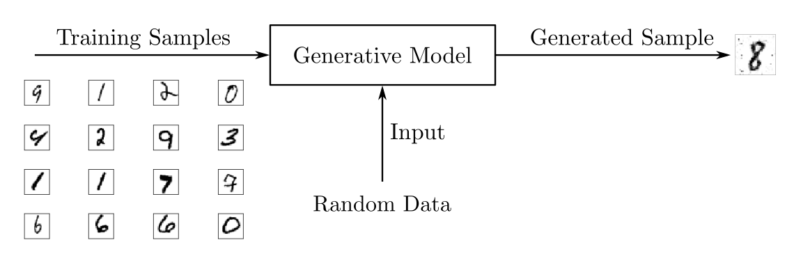
To output new samples, generative models usually consider a stochastic, or random, element that influences the samples generated by the model. The random samples used to drive the generator are obtained from a latent space in which the vectors represent a kind of compressed form of the generated samples.

Unlike discriminative models, generative models learn the probability P(x) of the input data x, and by having the distribution of the input data, they’re able to generate new data instances.

Note: Generative models can also be used with labeled datasets. When they are, they’re trained to learn the probability P(x|y) of the input x given the output y. They can also be used for classification tasks, but in general, discriminative models perform better when it comes to classification.

You can find more information on the relative strengths and weaknesses of discriminative and generative classifiers in the article On Discriminative vs. Generative Classifiers: A comparison of logistic regression and naive Bayes.

Although GANs have received a lot of attention in recent years, they’re not the only architecture that can be used as a generative model. Besides GANs, there are various other generative model architectures such as:

Boltzmann machines
Variational autoencoders
Hidden Markov models
Models that predict the next word in a sequence, like GPT-2

However, GANs have attracted the most public interest of late due to the exciting results in image and video generation.

Now that you know the basics of generative models, you’ll see how GANs work and how to train them.

The Architecture of Generative Adversarial Networks

Generative adversarial networks consist of an overall structure composed of two neural networks, one called the generator and the other called the discriminator.

The role of the generator is to estimate the probability distribution of the real samples in order to provide generated samples resembling real data. The discriminator, in turn, is trained to estimate the probability that a given sample came from the real data rather than being provided by the generator.

These structures are called generative adversarial networks because the generator and discriminator are trained to compete with each other: the generator tries to get better at fooling the discriminator, while the discriminator tries to get better at identifying generated samples.

To understand how GAN training works, consider a toy example with a dataset composed of two-dimensional samples (x₁, x₂), with x₁ in the interval from 0 to 2π and x₂ = sin(x₁), as illustrated in the following figure:

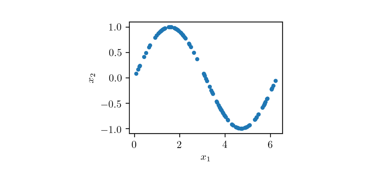
As you can see, this dataset consists of points (x₁, x₂) located over a sine curve, having a very particular distribution. The overall structure of a GAN to generate pairs (x̃₁, x̃₂) resembling the samples of the dataset is shown in the following figure:

The generator G is fed with random data from a latent space, and its role is to generate data resembling the real samples. In this example, you have a two-dimensional latent space, so that the generator is fed with random (z₁, z₂) pairs and is required to transform them so that they resemble the real samples.

The structure of the neural network G can be arbitrary, allowing you to use neural networks as a multilayer perceptron (MLP), a convolutional neural network (CNN), or any other structure as long as the dimensions of the input and output match the dimensions of the latent space and the real data.

The discriminator D is fed with either real samples from the training dataset or generated samples provided by G. Its role is to estimate the probability that the input belongs to the real dataset. The training is performed so that D outputs 1 when it’s fed a real sample and 0 when it’s fed a generated sample.

As with G, you can choose an arbitrary neural network structure for D as long as it respects the necessary input and output dimensions. In this example, the input is two-dimensional. For a binary discriminator, the output may be a scalar ranging from 0 to 1.

The GAN training process consists of a two-player minimax game in which D is adapted to minimize the discrimination error between real and generated samples, and G is adapted to maximize the probability of D making a mistake.

Although the dataset containing the real data isn’t labeled, the training processes for D and G are performed in a supervised way. At each step in the training, D and G have their parameters updated. In fact, in the original GAN proposal, the parameters of D are updated k times, while the parameters of G are updated only once for each training step. However, to make the training simpler, you can consider k equal to 1.

To train D, at each iteration you label some real samples taken from the training data as 1 and some generated samples provided by G as 0. This way, you can use a conventional supervised training framework to update the parameters of D in order to minimize a loss function, as shown in the following scheme:

For each batch of training data containing labeled real and generated samples, you update the parameters of D to minimize a loss function. After the parameters of D are updated, you train G to produce better generated samples. The output of G is connected to D, whose parameters are kept frozen, as depicted here:

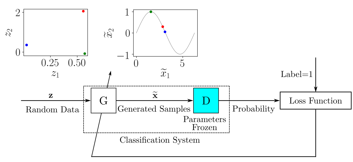
You can imagine the system composed of G and D as a single classification system that receives random samples as input and outputs the classification, which in this case can be interpreted as a probability.

When G does a good enough job to fool D, the output probability should be close to 1. You could also use a conventional supervised training framework here: the dataset to train the classification system composed of G and D would be provided by random input samples, and the label associated with each input sample would be 1.

During training, as the parameters of D and G are updated, it’s expected that the generated samples given by G will more closely resemble the real data, and D will have more trouble distinguishing between real and generated data.

Now that you know how GANs work, you’re ready to implement your own using PyTorch.

Remove ads

Your First GAN

As a first experiment with generative adversarial networks, you’ll implement the example described in the previous section.

To run the example, you’re going to use the PyTorch library, which you can install using the Anaconda Python distribution and the conda package and environment management system. To learn more about Anaconda and conda, check out the tutorial on Setting Up Python for Machine Learning on Windows.

To begin, create a conda environment and activate it:

Shell
      
$ conda create --name gan
$ conda activate gan

After you activate the conda environment, your prompt will show its name, gan. Then you can install the necessary packages inside the environment:

Shell
      
$ conda install -c pytorch pytorch=1.4.0
$ conda install matplotlib jupyter

Since PyTorch is a very actively developed framework, the API may change on new releases. To ensure the example code will run, you install the specific version 1.4.0.

Besides PyTorch, you’re going to use Matplotlib to work with plots and a Jupyter Notebook to run the code in an interactive environment. Doing so isn’t mandatory, but it facilitates working on machine learning projects.

For a refresher on working with Matplotlib and Jupyter Notebooks, take a look at Python Plotting With Matplotlib (Guide) and Jupyter Notebook: An Introduction.

Before opening Jupyter Notebook, you need to register the conda gan environment so that you can create Notebooks using it as the kernel. To do that, with the gan environment activated, run the following command:

Shell
      
$ python -m ipykernel install --user --name gan

Now you can open Jupyter Notebook by running jupyter notebook. Create a new Notebook by clicking New and then selecting gan.

Inside the Notebook, begin by importing the necessary libraries:

Python
      
    
import torch
from torch import nn

import math
import matplotlib.pyplot as plt

Here, you import the PyTorch library with torch. You also import nn just to be able to set up the neural networks in a less verbose way. Then you import math to obtain the value of the pi constant, and you import the Matplotlib plotting tools as plt as usual.

It’s a good practice to set up a random generator seed so that the experiment can be replicated identically on any machine. To do that in PyTorch, run the following code:

Python
      
torch.manual_seed(111)

The number 111 represents the random seed used to initialize the random number generator, which is used to initialize the neural network’s weights. Despite the random nature of the experiment, it must provide the same results as long as the same seed is used.

Now that the environment is set, you can prepare the training data.

Remove ads

Preparing the Training Data

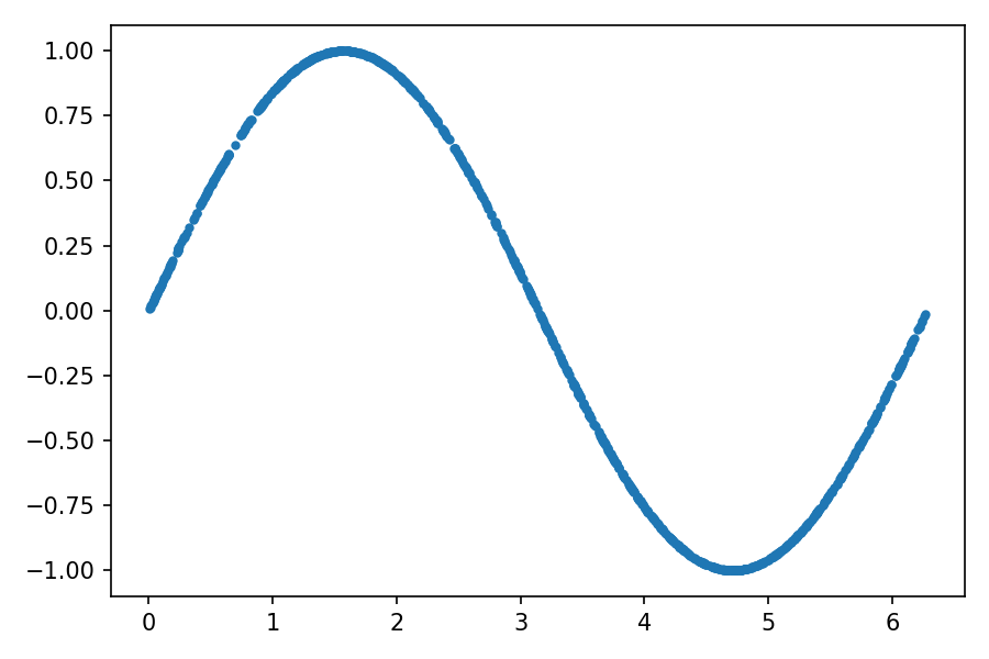
The training data is composed of pairs (x₁, x₂) so that x₂ consists of the value of the sine of x₁ for x₁ in the interval from 0 to 2π. You can implement it as follows:

Python
      
    
train_data_length = 1024
train_data = torch.zeros((train_data_length, 2))
train_data[:, 0] = 2 * math.pi * torch.rand(train_data_length)
train_data[:, 1] = torch.sin(train_data[:, 0])
train_labels = torch.zeros(train_data_length)
train_set = [
    (train_data[i], train_labels[i]) for i in range(train_data_length)
]

Here, you compose a training set with 1024 pairs (x₁, x₂). In line 2, you initialize train_data, a tensor with dimensions of 1024 rows and 2 columns, all containing zeros. A tensor is a multidimensional array similar to a NumPy array.

In line 3, you use the first column of train_data to store random values in the interval from 0 to 2π. Then, in line 4, you calculate the second column of the tensor as the sine of the first column.

Next, you’ll need a tensor of labels, which are required by PyTorch’s data loader. Since GANs make use of unsupervised learning techniques, the labels can be anything. They won’t be used, after all.

In line 5, you create train_labels, a tensor filled with zeros. Finally, in lines 6 to 8, you create train_set as a list of tuples, with each row of train_data and train_labels represented in each tuple as expected by PyTorch’s data loader.

You can examine the training data by plotting each point (x₁, x₂):

Python
      
plt.plot(train_data[:, 0], train_data[:, 1], ".")

The output should be something similar to the following figure:

With train_set, you can create a PyTorch data loader:

Python
      
    
batch_size = 32
train_loader = torch.utils.data.DataLoader(
    train_set, batch_size=batch_size, shuffle=True
)

Here, you create a data loader called train_loader, which will shuffle the data from train_set and return batches of 32 samples that you’ll use to train the neural networks.

After setting up the training data, you need to create the neural networks for the discriminator and generator that will compose the GAN. In the following section, you’ll implement the discriminator.

Implementing the Discriminator

In PyTorch, the neural network models are represented by classes that inherit from nn.Module, so you’ll have to define a class to create the discriminator. For more information on defining classes, take a look at Object-Oriented Programming (OOP) in Python 3.

The discriminator is a model with a two-dimensional input and a one-dimensional output. It’ll receive a sample from the real data or from the generator and will provide the probability that the sample belongs to the real training data. The code below shows how to create a discriminator:

Python
      
    
class Discriminator(nn.Module):
    def __init__(self):
        super().__init__()
        self.model = nn.Sequential(
            nn.Linear(2, 256),
            nn.ReLU(),
            nn.Dropout(0.3),
            nn.Linear(256, 128),
            nn.ReLU(),
            nn.Dropout(0.3),
            nn.Linear(128, 64),
            nn.ReLU(),
            nn.Dropout(0.3),
            nn.Linear(64, 1),
            nn.Sigmoid(),
        )

    def forward(self, x):
        output = self.model(x)
        return output

You use .__init__() to build the model. First, you need to call super().__init__() to run .__init__() from nn.Module. The discriminator you’re using is an MLP neural network defined in a sequential way using nn.Sequential(). It has the following characteristics:

Lines 5 and 6: The input is two-dimensional, and the first hidden layer is composed of 256 neurons with ReLU activation.
Lines 8, 9, 11, and 12: The second and third hidden layers are composed of 128 and 64 neurons, respectively, with ReLU activation.
Lines 14 and 15: The output is composed of a single neuron with sigmoidal activation to represent a probability.
Lines 7, 10, and 13: After the first, second, and third hidden layers, you use dropout to avoid overfitting.

Finally, you use .forward() to describe how the output of the model is calculated. Here, x represents the input of the model, which is a two-dimensional tensor. In this implementation, the output is obtained by feeding the input x to the model you’ve defined without any other processing.

After declaring the discriminator class, you should instantiate a Discriminator object:

Python
      
discriminator = Discriminator()

discriminator represents an instance of the neural network you’ve defined and is ready to be trained. However, before you implement the training loop, your GAN also needs a generator. You’ll implement one in the next section.

Remove ads

Implementing the Generator

In generative adversarial networks, the generator is the model that takes samples from a latent space as its input and generates data resembling the data in the training set. In this case, it’s a model with a two-dimensional input, which will receive random points (z₁, z₂), and a two-dimensional output that must provide (x̃₁, x̃₂) points resembling those from the training data.

The implementation is similar to what you did for the discriminator. First, you have to create a Generator class that inherits from nn.Module, defining the neural network architecture, and then you need instantiate a Generator object:

Python
      
    
class Generator(nn.Module):
    def __init__(self):
        super().__init__()
        self.model = nn.Sequential(
            nn.Linear(2, 16),
            nn.ReLU(),
            nn.Linear(16, 32),
            nn.ReLU(),
            nn.Linear(32, 2),
        )

    def forward(self, x):
        output = self.model(x)
        return output

generator = Generator()

Here, generator represents the generator neural network. It’s composed of two hidden layers with 16 and 32 neurons, both with ReLU activation, and a linear activation layer with 2 neurons in the output. This way, the output will consist of a vector with two elements that can be any value ranging from negative infinity to infinity, which will represent (x̃₁, x̃₂).

Now that you’ve defined the models for the discriminator and generator, you’re ready to perform the training!

Training the Models

Before training the models, you need to set up some parameters to use during training:

Python
      
    
lr = 0.001
num_epochs = 300
loss_function = nn.BCELoss()

Here you set up the following parameters:

Line 1 sets the learning rate (lr), which you’ll use to adapt the network weights.
Line 2 sets the number of epochs (num_epochs), which defines how many repetitions of training using the whole training set will be performed.
Line 3 assigns the variable loss_function to the binary cross-entropy function BCELoss(), which is the loss function that you’ll use to train the models.

The binary cross-entropy function is a suitable loss function for training the discriminator because it considers a binary classification task. It’s also suitable for training the generator since it feeds its output to the discriminator, which provides a binary observable output.

PyTorch implements various weight update rules for model training in torch.optim. You’ll use the Adam algorithm to train the discriminator and generator models. To create the optimizers using torch.optim, run the following lines:

Python
      
    
optimizer_discriminator = torch.optim.Adam(discriminator.parameters(), lr=lr)
optimizer_generator = torch.optim.Adam(generator.parameters(), lr=lr)

Finally, you need to implement a training loop in which training samples are fed to the models, and their weights are updated to minimize the loss function:

Python
      
    
for epoch in range(num_epochs):
    for n, (real_samples, _) in enumerate(train_loader):
        # Data for training the discriminator
        real_samples_labels = torch.ones((batch_size, 1))
        latent_space_samples = torch.randn((batch_size, 2))
        generated_samples = generator(latent_space_samples)
        generated_samples_labels = torch.zeros((batch_size, 1))
        all_samples = torch.cat((real_samples, generated_samples))
        all_samples_labels = torch.cat(
            (real_samples_labels, generated_samples_labels)
        )

        # Training the discriminator
        discriminator.zero_grad()
        output_discriminator = discriminator(all_samples)
        loss_discriminator = loss_function(
            output_discriminator, all_samples_labels)
        loss_discriminator.backward()
        optimizer_discriminator.step()

        # Data for training the generator
        latent_space_samples = torch.randn((batch_size, 2))

        # Training the generator
        generator.zero_grad()
        generated_samples = generator(latent_space_samples)
        output_discriminator_generated = discriminator(generated_samples)
        loss_generator = loss_function(
            output_discriminator_generated, real_samples_labels
        )
        loss_generator.backward()
        optimizer_generator.step()

        # Show loss
        if epoch % 10 == 0 and n == batch_size - 1:
            print(f"Epoch: {epoch} Loss D.: {loss_discriminator}")
            print(f"Epoch: {epoch} Loss G.: {loss_generator}")

For GANs, you update the parameters of the discriminator and the generator at each training iteration. As is generally done for all neural networks, the training process consists of two loops, one for the training epochs and the other for the batches for each epoch. Inside the inner loop, you begin preparing the data to train the discriminator:

Line 2: You get the real samples of the current batch from the data loader and assign them to real_samples. Notice that the first dimension of the tensor has the number of elements equal to batch_size. This is the standard way of organizing data in PyTorch, with each line of the tensor representing one sample from the batch.
Line 4: You use torch.ones() to create labels with the value 1 for the real samples, and then you assign the labels to real_samples_labels.
Lines 5 and 6: You create the generated samples by storing random data in latent_space_samples, which you then feed to the generator to obtain generated_samples.
Line 7: You use torch.zeros() to assign the value 0 to the labels for the generated samples, and then you store the labels in generated_samples_labels.
Lines 8 to 11: You concatenate the real and generated samples and labels and store them in all_samples and all_samples_labels, which you’ll use to train the discriminator.

Next, in lines 14 to 19, you train the discriminator:

Line 14: In PyTorch, it’s necessary to clear the gradients at each training step to avoid accumulating them. You do this using .zero_grad().
Line 15: You calculate the output of the discriminator using the training data in all_samples.
Lines 16 and 17: You calculate the loss function using the output from the model in output_discriminator and the labels in all_samples_labels.
Line 18: You calculate the gradients to update the weights with loss_discriminator.backward().
Line 19: You update the discriminator weights by calling optimizer_discriminator.step().

Next, in line 22, you prepare the data to train the generator. You store random data in latent_space_samples, with a number of lines equal to batch_size. You use two columns since you’re providing two-dimensional data as input to the generator.

You train the generator in lines 25 to 32:

Line 25: You clear the gradients with .zero_grad().
Line 26: You feed the generator with latent_space_samples and store its output in generated_samples.
Line 27: You feed the generator’s output into the discriminator and store its output in output_discriminator_generated, which you’ll use as the output of the whole model.
Lines 28 to 30: You calculate the loss function using the output of the classification system stored in output_discriminator_generated and the labels in real_samples_labels, which are all equal to 1.
Lines 31 and 32: You calculate the gradients and update the generator weights. Remember that when you trained the generator, you kept the discriminator weights frozen since you created optimizer_generator with its first argument equal to generator.parameters().

Finally, on lines 35 to 37, you display the values of the discriminator and generator loss functions at the end of each ten epochs.

Since the models used in this example have few parameters, the training will be complete in a few minutes. In the following section, you’ll use the trained GAN to generate some samples.

Remove ads

Checking the Samples Generated by the GAN

Generative adversarial networks are designed to generate data. So, after the training process is finished, you can get some random samples from the latent space and feed them to the generator to obtain some generated samples:

Python
      
    
latent_space_samples = torch.randn(100, 2)
generated_samples = generator(latent_space_samples)

Then you can plot the generated samples and check if they resemble the training data. Before plotting the generated_samples data, you’ll need to use .detach() to return a tensor from the PyTorch computational graph, which you’ll then use to calculate the gradients:

Python
      
    
generated_samples = generated_samples.detach()
plt.plot(generated_samples[:, 0], generated_samples[:, 1], ".")

The output should be similar to the following figure:

You can see the distribution of the generated data resembles the one from the real data. By using a fixed latent space samples tensor and feeding it to the generator at the end of each epoch during the training process, you can visualize the evolution of the training:

Note that at the beginning of the training process, the generated data distribution is very different from the real data. However, as the training progresses, the generator learns the real data distribution.

Now that you’ve done your first implementation of a generative adversarial network, you’ll go through a more practical application using images.

Handwritten Digits Generator With a GAN

Generative adversarial networks can also generate high-dimensional samples such as images. In this example, you’re going to use a GAN to generate images of handwritten digits. For that, you’ll train the models using the MNIST dataset of handwritten digits, which is included in the torchvision package.

To begin, you need to install torchvision in the activated gan conda environment:

Shell
      
$ conda install -c pytorch torchvision=0.5.0

Again, you’re using a specific version of torchvision to assure the example code will run, just like you did with pytorch. With the environment set up, you can start implementing the models in Jupyter Notebook. Open it and create a new Notebook by clicking on New and then selecting gan.

As in the previous example, you start by importing the necessary libraries:

Python
      
    
import torch
from torch import nn

import math
import matplotlib.pyplot as plt
import torchvision
import torchvision.transforms as transforms

Besides the libraries you’ve imported before, you’re going to need torchvision and transforms to obtain the training data and perform image conversions.

Again, set up the random generator seed to be able to replicate the experiment:

Python
      
torch.manual_seed(111)

Since this example uses images in the training set, the models need to be more complex, with a larger number of parameters. This makes the training process slower, taking about two minutes per epoch when running on CPU. You’ll need about fifty epochs to obtain a relevant result, so the total training time when using a CPU is around one hundred minutes.

To reduce the training time, you can use a GPU to train the model if you have one available. However, you’ll need to manually move tensors and models to the GPU in order to use them in the training process.

You can ensure your code will run on either setup by creating a device object that points either to the CPU or, if one is available, to the GPU:

Python
      
    
device = ""
if torch.cuda.is_available():
    device = torch.device("cuda")
else:
    device = torch.device("cpu")

Later, you’ll use this device to set where tensors and models should be created, using the GPU if available.

Now that the basic environment is set, you can prepare the training data.

Remove ads

Preparing the Training Data

The MNIST dataset consists of 28 × 28 pixel grayscale images of handwritten digits from 0 to 9. To use them with PyTorch, you’ll need to perform some conversions. For that, you define transform, a function to be used when loading the data:

Python
      
    
transform = transforms.Compose(
    [transforms.ToTensor(), transforms.Normalize((0.5,), (0.5,))]
)

The function has two parts:

transforms.ToTensor() converts the data to a PyTorch tensor.
transforms.Normalize() converts the range of the tensor coefficients.

The original coefficients given by transforms.ToTensor() range from 0 to 1, and since the image backgrounds are black, most of the coefficients are equal to 0 when they’re represented using this range.

transforms.Normalize() changes the range of the coefficients to -1 to 1 by subtracting 0.5 from the original coefficients and dividing the result by 0.5. With this transformation, the number of elements equal to 0 in the input samples is dramatically reduced, which helps in training the models.

The arguments of transforms.Normalize() are two tuples, (M₁, ..., Mₙ) and (S₁, ..., Sₙ), with n representing the number of channels of the images. Grayscale images such as those in MNIST dataset have only one channel, so the tuples have only one value. Then, for each channel i of the image, transforms.Normalize() subtracts Mᵢ from the coefficients and divides the result by Sᵢ.

Now you can load the training data using torchvision.datasets.MNIST and perform the conversions using transform:

Python
      
    
train_set = torchvision.datasets.MNIST(
    root=".", train=True, download=True, transform=transform
)

The argument download=True ensures that the first time you run the above code, the MNIST dataset will be downloaded and stored in the current directory, as indicated by the argument root.

Now that you’ve created train_set, you can create the data loader as you did before:

Python
      
    
batch_size = 32
train_loader = torch.utils.data.DataLoader(
    train_set, batch_size=batch_size, shuffle=True
)

You can use Matplotlib to plot some samples of the training data. To improve the visualization, you can use cmap=gray_r to reverse the color map and plot the digits in black over a white background:

Python
      
    
real_samples, mnist_labels = next(iter(train_loader))
for i in range(16):
    ax = plt.subplot(4, 4, i + 1)
    plt.imshow(real_samples[i].reshape(28, 28), cmap="gray_r")
    plt.xticks([])
    plt.yticks([])

The output should be something similar to the following:

As you can see, there are digits with different handwriting styles. As the GAN learns the distribution of the data, it’ll also generate digits with different handwriting styles.

Now that you’ve prepared the training data, you can implement the discriminator and generator models.

Implementing the Discriminator and the Generator

In this case, the discriminator is an MLP neural network that receives a 28 × 28 pixel image and provides the probability of the image belonging to the real training data.

You can define the model with the following code:

Python
      
    
class Discriminator(nn.Module):
    def __init__(self):
        super().__init__()
        self.model = nn.Sequential(
            nn.Linear(784, 1024),
            nn.ReLU(),
            nn.Dropout(0.3),
            nn.Linear(1024, 512),
            nn.ReLU(),
            nn.Dropout(0.3),
            nn.Linear(512, 256),
            nn.ReLU(),
            nn.Dropout(0.3),
            nn.Linear(256, 1),
            nn.Sigmoid(),
        )

    def forward(self, x):
        x = x.view(x.size(0), 784)
        output = self.model(x)
        return output

To input the image coefficients into the MLP neural network, you vectorize them so that the neural network receives vectors with 784 coefficients.

The vectorization occurs in the first line of .forward(), as the call to x.view() converts the shape of the input tensor. In this case, the original shape of the input x is 32 × 1 × 28 × 28, where 32 is the batch size you’ve set up. After the conversion, the shape of x becomes 32 × 784, with each line representing the coefficients of an image of the training set.

To run the discriminator model using the GPU, you have to instantiate it and send it to the GPU with .to(). To use a GPU when there’s one available, you can send the model to the device object you created earlier:

Python
      
discriminator = Discriminator().to(device=device)

Since the generator is going to generate more complex data, it’s necessary to increase the dimensions of the input from the latent space. In this case, the generator is going to be fed a 100-dimensional input and will provide an output with 784 coefficients, which will be organized in a 28 × 28 tensor representing an image.

Here’s the complete generator model code:

Python
      
    
class Generator(nn.Module):
    def __init__(self):
        super().__init__()
        self.model = nn.Sequential(
            nn.Linear(100, 256),
            nn.ReLU(),
            nn.Linear(256, 512),
            nn.ReLU(),
            nn.Linear(512, 1024),
            nn.ReLU(),
            nn.Linear(1024, 784),
            nn.Tanh(),
        )

    def forward(self, x):
        output = self.model(x)
        output = output.view(x.size(0), 1, 28, 28)
        return output

generator = Generator().to(device=device)

In line 12, you use the hyperbolic tangent function Tanh() as the activation of the output layer since the output coefficients should be in the interval from -1 to 1. In line 20, you instantiate the generator and send it to device to use the GPU if one is available.

Now that you have the models defined, you’ll train them using the training data.

Remove ads

Training the Models

To train the models, you need to define the training parameters and optimizers like you did in the previous example:

Python
      
    
lr = 0.0001
num_epochs = 50
loss_function = nn.BCELoss()

optimizer_discriminator = torch.optim.Adam(discriminator.parameters(), lr=lr)
optimizer_generator = torch.optim.Adam(generator.parameters(), lr=lr)

To obtain a better result, you decrease the learning rate from the previous example. You also set the number of epochs to 50 to reduce the training time.

The training loop is very similar to the one you used in the previous example. In the highlighted lines, you send the training data to device to use the GPU if available:

Python
      
    
for epoch in range(num_epochs):
    for n, (real_samples, mnist_labels) in enumerate(train_loader):
        # Data for training the discriminator
        real_samples = real_samples.to(device=device)
        real_samples_labels = torch.ones((batch_size, 1)).to(
            device=device
        )
        latent_space_samples = torch.randn((batch_size, 100)).to(
            device=device
        )
        generated_samples = generator(latent_space_samples)
        generated_samples_labels = torch.zeros((batch_size, 1)).to(
            device=device
        )
        all_samples = torch.cat((real_samples, generated_samples))
        all_samples_labels = torch.cat(
            (real_samples_labels, generated_samples_labels)
        )

        # Training the discriminator
        discriminator.zero_grad()
        output_discriminator = discriminator(all_samples)
        loss_discriminator = loss_function(
            output_discriminator, all_samples_labels
        )
        loss_discriminator.backward()
        optimizer_discriminator.step()

        # Data for training the generator
        latent_space_samples = torch.randn((batch_size, 100)).to(
            device=device
        )

        # Training the generator
        generator.zero_grad()
        generated_samples = generator(latent_space_samples)
        output_discriminator_generated = discriminator(generated_samples)
        loss_generator = loss_function(
            output_discriminator_generated, real_samples_labels
        )
        loss_generator.backward()
        optimizer_generator.step()

        # Show loss
        if n == batch_size - 1:
            print(f"Epoch: {epoch} Loss D.: {loss_discriminator}")
            print(f"Epoch: {epoch} Loss G.: {loss_generator}")

Some of the tensors don’t need to be sent to the GPU explicitly with device. This is the case with generated_samples in line 11, which will already be sent to an available GPU since latent_space_samples and generator were sent to the GPU previously.

Since this example features more complex models, the training may take a bit more time. After it finishes, you can check the results by generating some samples of handwritten digits.

Checking the Samples Generated by the GAN

To generate handwritten digits, you have to take some random samples from the latent space and feed them to the generator:

Python
      
    
latent_space_samples = torch.randn(batch_size, 100).to(device=device)
generated_samples = generator(latent_space_samples)

To plot generated_samples, you need to move the data back to the CPU in case it’s running on the GPU. For that, you can simply call .cpu(). As you did previously, you also need to call .detach() before using Matplotlib to plot the data:

Python
      
    
generated_samples = generated_samples.cpu().detach()
for i in range(16):
    ax = plt.subplot(4, 4, i + 1)
    plt.imshow(generated_samples[i].reshape(28, 28), cmap="gray_r")
    plt.xticks([])
    plt.yticks([])

The output should be digits resembling the training data, as in the following figure:

After fifty epochs of training, there are several generated digits that resemble the real ones. You can improve the results by considering more training epochs. As with the previous example, by using a fixed latent space samples tensor and feeding it to the generator at the end of each epoch during the training process, you can visualize the evolution of the training:

You can see that at the beginning of the training process, the generated images are completely random. As the training progresses, the generator learns the distribution of the real data, and at about twenty epochs, some generated digits already resemble real data.

Conclusion

Congratulations! You’ve learned how to implement your own generative adversarial networks. You first went through a toy example to understand the GAN structure before diving into a practical application that generates images of handwritten digits.

You saw that, despite the complexity of GANs, machine learning frameworks like PyTorch make the implementation more straightforward by offering automatic differentiation and easy GPU setup.

In this tutorial, you learned:

What the difference is between discriminative and generative models
How generative adversarial networks are structured and trained
How to use tools like PyTorch and a GPU to implement and train GAN models

GANs are a very active research topic, with several exciting applications proposed in recent years. If you’re interested in the subject, keep an eye on the technical and scientific literature to check for new application ideas.

Remove ads