
Unlocking Python’s true potential in terms of speed through shared-memory parallelism has traditionally been limited and challenging to achieve. That’s because the global interpreter lock (GIL) doesn’t allow for thread-based parallel processing in Python. Fortunately, there are several work-arounds for this notorious limitation, which you’re about to explore now!
In this tutorial, you’ll learn how to:
- Run Python threads in parallel on multiple CPU cores
- Avoid the data serialization overhead of multiprocessing
- Share memory between Python and C runtime environments
- Use different strategies to bypass the GIL in Python
- Parallelize your Python programs to improve their performance
- Build a sample desktop application for parallel image processing
To get the most out of this advanced tutorial, you should understand the difference between concurrency and parallelism. You’ll benefit from having previous experience with multithreading in programming languages other than Python. Finally, it’s best if you’re eager to explore uncharted territory, such as calling foreign Python bindings or writing bits of C code.
Don’t worry if your knowledge of parallel processing is a bit rusty, as you’ll have a chance to quickly refresh your memory in the upcoming sections. Also, note that you’ll find all the code samples, image files, and the demo project from this tutorial in the supporting materials, which you can download below:
Get Your Code: Click here to download the free sample code that shows you how to bypass the GIL and achieve parallel processing in Python.
Recall the Fundamentals of Parallel Processing
Before dipping your toes into specific ways of bypassing the GIL in Python, you might want to revisit some related topics. Over the following few sections, you’ll familiarize yourself with different computer processing models, task types, abstractions over modern CPUs, and some history. If you already know this information, then feel free to jump ahead to the classic mechanism for parallelization in Python.
What’s Parallel Processing?
Under Flynn’s taxonomy, the most common types of parallel processing allow you to run the same (SIMD) or different code fragments (MIMD) in separate execution streams at the same time:
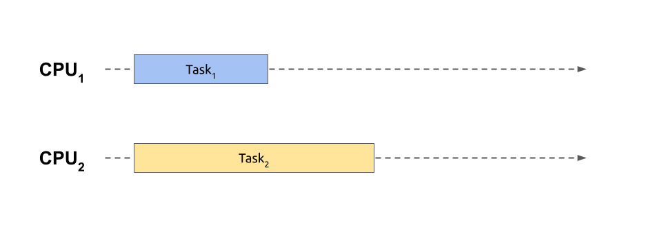
Here, two independent tasks or jobs execute alongside each other. To run more than one piece of code simultaneously like this, you need a computer equipped with a central processing unit (CPU) comprising multiple physical cores, which is the norm nowadays. While you could alternatively access a cluster of geographically distributed machines, you’ll consider only the first option in this tutorial.
Parallel processing is a particular form of concurrent processing, which is a broader term encompassing context switching between multiple tasks. It means that a currently running task might voluntarily suspend its execution or be forcibly suspended to give a slice of the CPU time to another task:
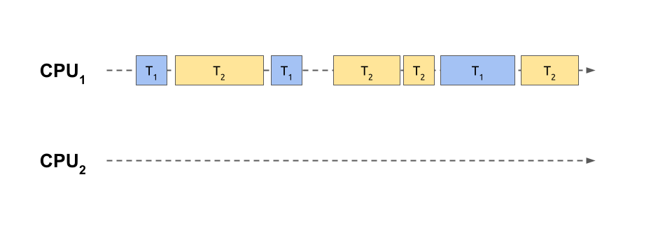
In this case, two tasks have been sliced into smaller and intertwined chunks of work that share a single core of the same processing unit. This is analogous to playing chess against multiple opponents at the same time, as shown in one of the scenes from the popular TV miniseries The Queen’s Gambit. After each move, the player proceeds to the next opponent in a round-robin fashion, trying to remember the state of the corresponding game.
Note: Context switching makes multitasking possible on single-core architectures. However, multi-core CPUs also benefit from this technique when the tasks outnumber the available processing power, which is often the case. Therefore, concurrent processing usually involves spreading the individual task slices over many CPUs, combining the power of context switching and parallel processing.
While it takes time for people to switch their focus, computers take turns much quicker. Rapid context switching gives the illusion of parallel execution despite using only one physical CPU. As a result, multiple tasks are making progress together.
Because of time-sharing, the total time required to finish your intertwined tasks running concurrently is longer when compared to a genuinely parallel version. In fact, context switching has a noticeable overhead that makes the execution time even worse than if you run your tasks one after another using sequential processing on a single CPU. Here’s what sequential processing looks like:
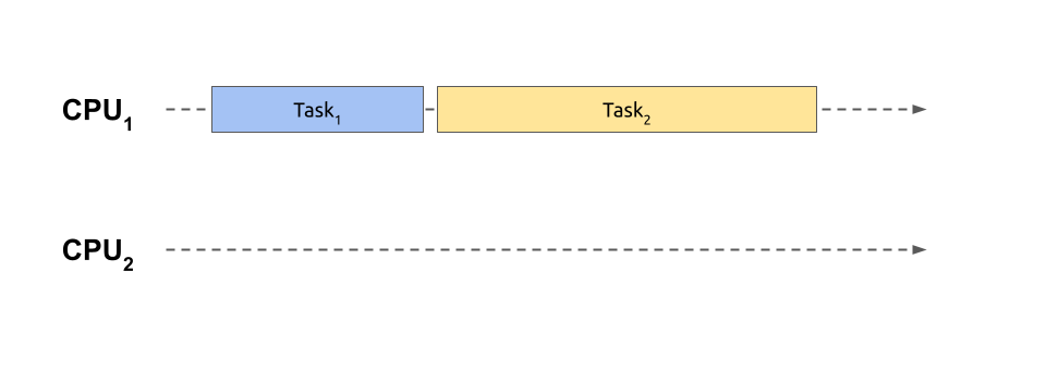
With sequential processing, you don’t start another task until the previous one finishes, so you don’t have the costs of switching back and forth. This situation corresponds to playing an entire chess game with one opponent before moving on to the next one. Meanwhile, the remaining players must sit tight, patiently waiting for their turn.
On the other hand, playing multiple games concurrently can maximize your throughput. When you prioritize games with players who make quick decisions over those who need more time to think, then you’ll finish more games sooner. Therefore, intertwining can improve the latency, or response times, of the individual tasks, even when you only have one stream of execution.
As you can probably tell, choosing between parallel, concurrent, and sequential processing models can feel like plotting out your next three moves in chess. You have to consider several factors, so there’s no one-size-fits-all solution.
Whether context switching actually helps will depend on how you prioritize your tasks. Inefficient task scheduling can lead to starving shorter tasks of CPU time.
Additionally, the types of tasks are critical. Two broad categories of concurrent tasks are CPU-bound and I/O-bound ones. The CPU-bound tasks will only benefit from truly parallel execution to run faster, whereas I/O-bound tasks can leverage concurrent processing to reduce latency. You’ll learn more about these categories’ characteristics now.
How Do CPU-Bound and I/O-Bound Tasks Differ?
Several factors can limit the pace at which concurrent tasks make progress. You’ll want to identify these bottlenecks before deciding whether parallel processing is appropriate for your needs and how to use it to your advantage.
The speed of a task performing heavy computations depends mainly on the clock rate of your CPU, which directly corresponds to the number of machine code instructions executed per unit of time. In other words, the faster your processor can run, the more work it’ll be able to do in the same amount of time. If your processor limits a task’s performance, then that task is said to be CPU bound.
When you only have CPU-bound tasks, then you’ll achieve better performance by running them in parallel on separate cores. However, that’ll only work up to a certain point before your tasks start competing for limited resources, and then the overhead associated with context switching will become troublesome. Generally, to avoid a slowdown, you shouldn’t simultaneously run more CPU-bound tasks than your CPU count.
Note: If you do have more CPU-bound tasks, then consider enqueuing them or using a pool of workers, such as a thread pool.
In theory, you should observe a linear growth of the overall speed, or a linear decrease in the total execution time, with each additional CPU. However, that isn’t a universal rule because different tasks may sometimes have varying amounts of work to do.
The CPU isn’t the only limiting factor out there. Tasks that spend most of their time waiting for data from a hard drive, a network, or a database don’t use all that much CPU time. The operating system can put them on hold and wake them up when a chunk of data arrives. These tasks are known as I/O bound because their performance is related to the throughput of the underlying input/output device.
Think of an I/O-bound task as playing chess against one particular opponent. You only need to make your move once in a while and then let the other player do the same. While they’re thinking, you can either wait or do something productive. For example, you can resume playing another game with a different player or make an urgent phone call.
As a result, you don’t have to run I/O-bound tasks in parallel to move them forward simultaneously. This fact removes the limitation on the maximum number of concurrent tasks. Unlike their CPU-bound counterparts, I/O-bound tasks aren’t limited by the number of physical CPU cores. You can have as many I/O-bound tasks in your application as your memory allows. It’s not uncommon to encounter hundreds or even thousands of such tasks.
Coincidentally, memory can be yet another limiting factor in progressing with concurrent tasks, although less common. Memory-bound jobs depend on the available amount of computer memory and the speed of access to it. When you increase memory consumption, you’ll often improve the performance of your task and the other way around. This is known as the time–memory trade-off.
While there are other limiting factors in concurrent programming, the CPU and I/O devices are by far the most important. But why and when did parallel processing itself become so prevalent? To better understand its significance in the modern world, you’ll get some brief historical context in the next section.
Why Do Modern Computers Favor Parallelism?
Up until about the mid-2000s, the number of transistors in computer processors doubled roughly every two years, as predicted by Moore’s law. This increase resulted in continuous peformance improvement for new CPU models, which meant that you could just wait until computers became fast enough to handle computationally demanding tasks.
Unfortunately, the free lunch is over because stuffing more and more transistors onto a single chip isn’t physically or economically viable for the manufacturers anymore. The semiconductor industry has instead decided to shift to making multi-core processors that can handle several tasks simultaneously. The idea was to gain performance without making the CPU faster. In fact, the individual cores may be slower than some older single-core chips!
Note: Technically speaking, the total number of transistors in new CPUs still increases, but that increase is now spread out across separate cores. The rate at which new cores are added is much slower, though.
This change in the underlying hardware architecture forces you, as a programmer, to adapt your software design to a completely new paradigm. To take advantage of multiple CPU cores, you must now find ways to decompose a monolithic piece of code into pieces that can run in arbitrary order. Doing so presents many new challenges, such as task coordination and access synchronization for shared resources, that were previously not a concern.
Moreover, while some problems are inherently parallelizable or—to use technical jargon—embarrassingly parallel, many other tasks require you to execute them sequentially in steps. For example, finding the nth Fibonacci number requires you to compute previous numbers in that sequence first. Such limitations can make a parallel algorithm implementation difficult or sometimes impossible.
At this point, you understand the concept of parallel processing and its significance in modern computing. Your next step should be learning about the available tools that can enable you to leverage parallelism in your programs. But you’ll also need to know about their weak points.
How Can You Harness the Power of Multiple CPU Cores?
Various mechanisms expose the parallel nature of modern CPUs while offering different trade-offs. For example, you can run chunks of your code in separate system processes. This approach provides a high level of resource isolation and data consistency at the price of expensive data serialization. What does this mean in practice?
Processes are straightforward because they usually require little coordination or synchronization. But, due to their relatively high cost of creation and interprocess communication (IPC), you can only make a few before you start getting diminishing returns. It’s best to avoid passing around large amounts of data between processes because of the serialization overhead, which can outweigh the benefits of such parallelization.
When you need to run a greater number of parallel tasks or have a much bigger dataset to process, then threads are a far better option. Threads are more lightweight and quicker to create than processes. They share a common memory area, making serialization unnecessary and their communication cheaper. At the same time, they require careful coordination and synchronization to avoid race conditions or data corruption, which can be difficult.
But even threads won’t provide enough scalability at some point. Massively parallel applications like real-time messaging platforms or streaming services require the ability to manage tens of thousands of concurrent connections. In contrast, modern operating systems can handle up to a few thousand threads.
To run such a huge number of simultaneous tasks, you can use coroutines, which are even more lightweight units of execution than threads. Unlike threads and processes, they don’t require a preemptive task scheduler because they leverage cooperative multitasking by voluntarily suspending their execution at explicit points. This has its own pros and cons, which you can explore in a tutorial on asynchronous programming in Python.
Note: Processes and threads are by far the most common building blocks in parallel processing. Coroutines are also popular but more suitable for handling concurrent network connections.
Fibers and green threads are lesser-known alternatives to coroutines, sometimes called microthreads. They’re essentially threads with cooperative multitasking and threads scheduled by user-space code instead of the operating system, respectively.
In Python, you can use microthreads through third-party libraries, like greenlet or eventlet.
In this tutorial, you’ll focus primarily on multithreading as a way of improving your program’s performance through parallelism. Threads have traditionally been the standard mechanism for parallel processing in many programming languages. Unfortunately, using threads in Python can be tricky, as you’re about to find out.
Compare Multithreading in Python and Other Languages
Multithreading usually entails splitting data, distributing the workload evenly over the available CPUs, coordinating the individual workers, synchronizing access to shared resources, and merging partial results. However, you won’t bother with any of that now. To illustrate the jarring problem with threads in Python, you’ll simultaneously call the same function on all the available CPU cores, ignoring the return value.
Java Threads Solve CPU-Bound and I/O-Bound Problems
You’re going to use Java in this section, but you could pick any other programming language with support for threads native to the operating system. The Java Development Kit (JDK) most likely didn’t ship with your computer, so you may need to install it. You can choose from a few implementations of the Java platform, including the official Oracle Java and OpenJDK.
Note: Alternatively, you can find a suitable Docker image with Java already installed.
For demonstration purposes, you’ll implement a recursive algorithm for finding the nth number of the Fibonacci sequence. The formula behind it is straightforward and elegant while being computationally expensive at the same time, which makes it a perfect benchmark for a CPU-bound problem:
// Fibonacci.java

public class Fibonacci {
    public static void main(String[] args) {
        int cpus = Runtime.getRuntime().availableProcessors();
        for (int i = 0; i < cpus; i++) {
            new Thread(() -> fib(45)).start();
        }
    }
    private static int fib(int n) {
        return n < 2 ? n : fib(n - 2) + fib(n - 1);
    }
}
You call the fib() method in separate threads of execution, creating as many threads as your CPU count. The input value of forty-five should be plenty to keep your computer busy, but if you have a beefy machine, then you might tweak the number accordingly. Don’t underestimate this seemingly basic code, though. Your method keeps calling itself until it reaches one of the base cases, draining a lot of CPU power for relatively small input values.
Note: Because each function call branches into two new ones until reaching the base case, the recursive implementation of fib() has exponential time complexity. In other words, the amount of work required to calculate the given Fibonacci number doesn’t grow linearly as the input value increases. For example, calling fib(45) is about 123 times more expensive than fib(35) despite the input value increasing by only 29 percent.
Although you could run your Java source code directly using the java command—or use the interactive JShell tool equivalent to Python’s REPL—you don’t want to measure the compilation step. Therefore, it’s best to compile the Java code in a separate command, producing a local .class file with the corresponding Java bytecode:
$ javac Fibonacci.java
$ time java Fibonacci

real    0m9.758s
user    0m38.465s
sys     0m0.020s
First, you compile the source code with a Java compiler (javac) that came with your JDK, and then time the execution of the resulting program.
According to the output above, your program took about 9.8 seconds to complete, as indicated by the elapsed real time. But notice the highlighted line directly below that, which represents the user time, or the total number of CPU seconds spent in all threads. The total CPU time was almost four times greater than the real time in this example, implying that your threads were running in parallel.
That’s great news! It means that you nearly quadrupled your program’s speed by leveraging Java’s multithreading. The performance improvement is close to but not exactly linear due to the overhead of creating and managing threads.
The CPU in question had two independent physical cores on board, which could each handle two threads in parallel thanks to Intel’s Hyper-Threading Technology. But you don’t generally need to be aware of such low-level technical details. From your perspective, there were four logical cores involved, which the operating system will report through its graphical user interface or command-line utility tools like nproc or lscpu.
Another way to prove that threads run in parallel is to inspect the CPU utilization with the help of a monitoring tool while your program is executing:
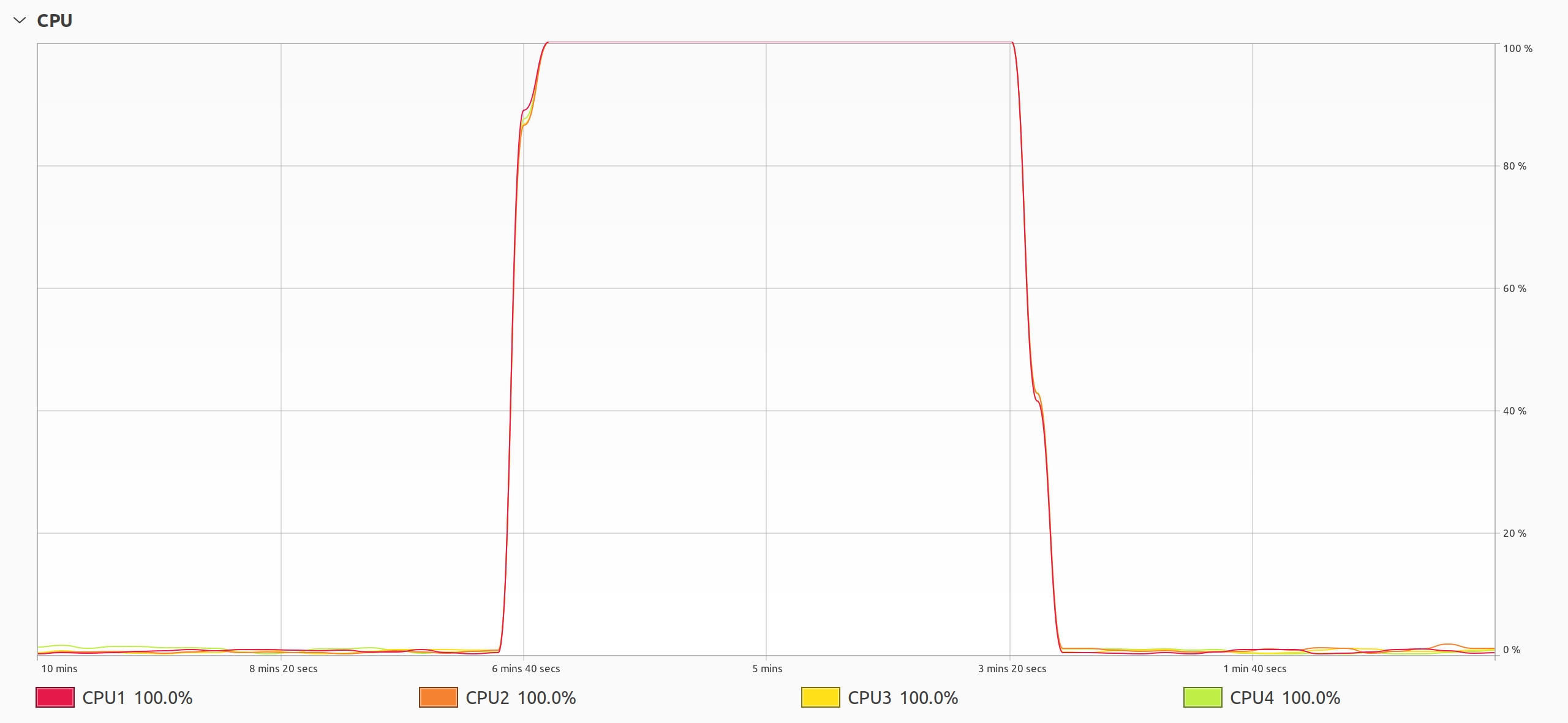
That’s the plot that you want to see when solving a CPU-bound problem using threads. As soon as you run your multithreaded program, all CPU cores suddenly start working at their full capacity until the program ends. You might even hear your computer’s fan spin up and feel it blow hot air as the processor works harder to keep up with the increased load.
In contrast, threads in Python behave quite differently, as you’re about to see.
Python Threads Only Solve I/O-Bound Problems
To make an apples-to-apples comparison, you’ll use the previous example. Go ahead and rewrite your Java implementation of the Fibonacci sequence into Python:
# fibonacci.py

import os
import threading

def fib(n):
    return n if n < 2 else fib(n - 2) + fib(n - 1)

for _ in range(os.cpu_count()):
    threading.Thread(target=fib, args=(35,)).start()
This code is nearly identical to its Java counterpart but uses Python syntax and the corresponding standard library bindings to threads. Also, the input argument to fib() is smaller to account for the fact that Python code runs orders of magnitude slower than Java. If you kept the same value as before, then the analogous Python code would run much longer, provided that you had enough patience to wait for it to finish.
Because Python is an interpreted language, you can run the above script directly without explicitly compiling it and measure the execution time:
$ time python3 fibonacci.py

real    0m8.754s
user    0m8.778s
sys     0m0.068s
Now, the elapsed time is essentially the same as the total CPU time. Despite creating and starting multiple threads, your program behaves as if it were single-threaded. What’s going on here?
To investigate this further, take a closer look at the CPU utilization of your Python script:
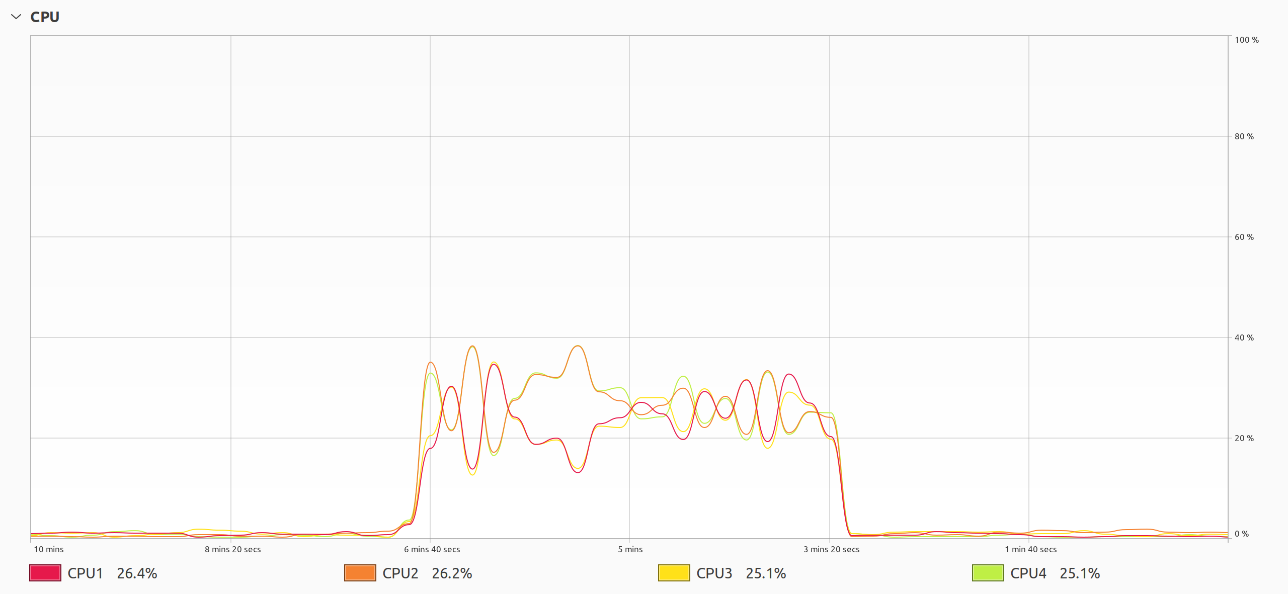
The plot reveals a peculiar behavior of threads in Python. Based on the measured timing, you could’ve expected just one CPU core to be working with maximum intensity, yet something more sinister is happening. All four CPU cores are performing computations, but they’re only operating at about a quarter of their potential. It’s almost as if you were using just one of the cores. But things get even more interesting than that.
The graphs of the individual cores have a perfectly symmetrical shape centered at around 25 percent, which is the average CPU utilization. The symmetry indicates a continuous migration of tasks across the processing units, which causes unnecessary context switching and resource contention. When multiple threads fight with each other for resources instead of working together toward a common goal, it severely decreases their overall performance.
Note: To some extent, you can control the shapes of these graphs by changing the switch interval, which determines the preferred duration of uninterrupted thread execution. However, this mechanism doesn’t give strict guarantees and relies on low-level implementation details that might change in the future.
The infamous global interpreter lock (GIL) is at play here, obstructing your attempts at parallel execution of Python code. The GIL only allows one thread to run at any given time, effectively turning your multithreaded program into a single-threaded one. At the same time, the operating system’s task scheduler tries to guess which of the threads should have the highest priority, moving it from one core to another.
Does that mean threads are completely useless in Python? Not exactly. They’re still appropriate for running I/O-bound tasks concurrently or for performing various kinds of simulations. Whenever a Python thread performs a blocking I/O operation, which may take some time to return, it’ll release the GIL and let other threads know they can now try acquiring the lock to resume execution.
The good news is that threads in Python absolutely have the potential to run in parallel, but the global interpreter lock inhibits them. Next, you’ll examine the GIL and threads in Python up close.
Python’s GIL Prevents Threads From Running in Parallel
Threads in Python are somewhat special. On the one hand, they’re full-fledged threads scheduled by the operating system, but on the other hand, they use cooperative multitasking, which is quite an unusual mix. Most systems today prefer time-sharing multitasking with a preemptive scheduler to ensure fair use of CPU time across the threads. Otherwise, greedy or poorly implemented workers could starve others.
The interpreter internally relies on the operating system’s threads exposed by libraries like POSIX threads. However, it allows only the single thread that currently holds the GIL to execute, which necessitates that threads periodically give up the GIL. As you learned earlier, an I/O operation will always trigger the thread to relinquish the GIL. Threads that don’t use any such operations will release the GIL anyway after a certain time period.
Before Python 3.2, the interpreter would release the GIL after executing a fixed number of bytecode instructions to give other threads a chance to run in case of no pending I/O operations. Because the scheduling was—and still is—done outside of Python by the operating system, the same thread that just released the GIL would often get it back immediately.
This mechanism made context switching incredibly wasteful and unfair. Plus, it was unpredictable because one bytecode instruction in Python can translate to a variable number of machine-code instructions with different associated costs. For example, a single call to a C function can take orders of magnitude longer than printing a newline, even though both are just one instruction.
The way the GIL is released and acquired has a surprising effect on your application’s performance. Oddly enough, you’ll get better performance of your CPU-bound threads in Python from running them on fewer CPU cores! Adding more may actually degrade performance. This was especially pronounced before Python 3.2, which introduced an overhauled GIL implementation to mitigate this problem.
Since then, instead of counting bytecodes, Python threads release the GIL after the switching interval, a specific time that defaults to five milliseconds. Note that it’s not precise, and it’ll only happen in the presence of other threads signaling the desire to grab the GIL for themselves.
Nevertheless, the new GIL hasn’t completely eliminated the undesired behavior. You can still observe the issue by setting the processor affinity for your Python script:
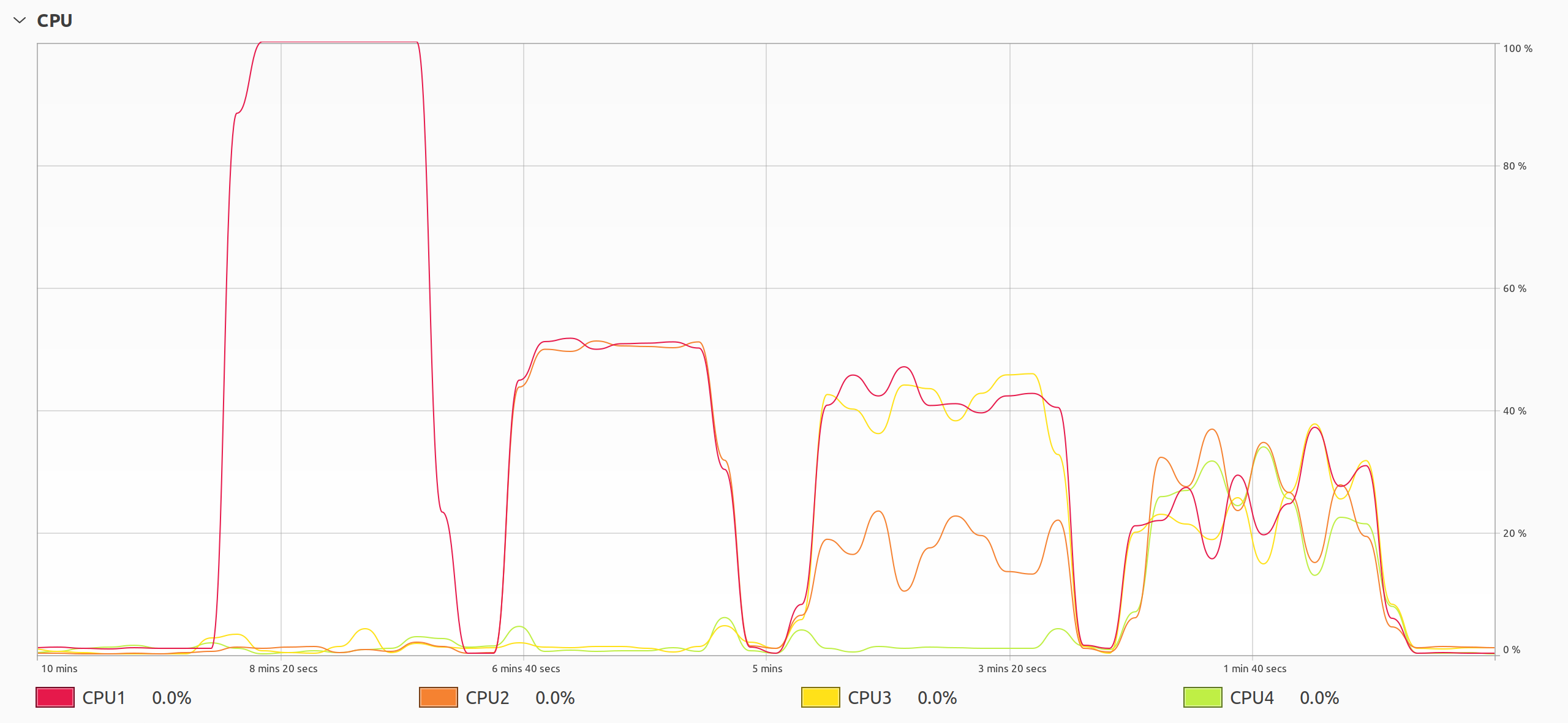
Looking from the left, you can see the effects of pinning your multithreaded Python program to one, two, three, and four CPU cores.
In the first case, one core is fully saturated while others remain dormant because the task scheduler doesn’t have much choice regarding CPU cores. When two CPU cores are active, they work at about half of their capacity. With three out of four cores, you end up with about one-third of the total CPU utilization on average, and you get a quarter with all four cores running. Do you recognize the familiar symmetrical shapes in the graphs?
If you’re on Linux, then you can use the taskset command to bind your program to one or more CPU cores:
$ time taskset --cpu-list 0 python3 fibonacci.py

real    0m6.992s
user    0m6.979s
sys     0m0.012s

$ time taskset --cpu-list 0,1 python3 fibonacci.py

real    0m9.509s
user    0m9.559s
sys     0m0.084s

$ time taskset --cpu-list 0,1,2 python3 fibonacci.py

real    0m9.527s
user    0m9.569s
sys     0m0.082s

$ time taskset --cpu-list 0,1,2,3 python3 fibonacci.py

real    0m9.619s
user    0m9.636s
sys     0m0.111s
While there’s no significant difference in the execution time when you use two or more CPU cores, the results are much better with just one core. This goes against common sense, but the GIL is again to blame.
If the GIL is so problematic for CPU-bound multithreaded programs, then why was it part of Python in the first place? You’ll get some insight in the next section.
The GIL Ensures Thread Safety of the Python Internals
Python wasn’t written with parallelism in mind. The language itself came into existence shortly before multithreading became a consideration, when most computers still had only one CPU on board. Because chip designers suddenly started pushing programmers to leverage threads in their code for better performance, lots of C libraries didn’t shy away from using them.
That became a real problem for Python, which couldn’t provide bindings for these emerging C libraries without ensuring thread safety first. Because of the underlying memory model and reference counting, running Python from multiple threads could lead to memory leaks or worse, crashing the program.
There were a few options on the table, but implementing the global interpreter lock seemed like a quick way to make the interpreter thread-safe, allowing the use of multithreaded C libraries.
One alternative was to rewrite the whole interpreter from scratch to make it thread-safe. However, it’d be a massive effort because everything in Python was written with the assumption that there’s ever only one thread. Moreover, this would introduce multiple locks instead of a global one, inevitably reducing the overall performance, especially of single-threaded code. Plus, it’d make Python’s code harder to understand and maintain.
On the other hand, the GIL provided a straightforward mechanism for anyone wishing to write a Python extension module using the Python/C API. According to Larry Hastings—who’s most famous for making Gilectomy, a GIL-free fork of Python—the GIL was the secret sauce behind Python’s success and popularity. It enabled the integration of Python with numerous C libraries in a short period of time.
While the GIL had its place in Python’s development, there have been several attempts to remove it over the years with various levels of success, including:
- free-threading by Greg Stein (Python 1.4)
- pypy-stm by Remi Meier and Armin Rigo (Python 2.5.1)
- python-safethread by Adam Olsen (Python 3.0b1)
- PyParallel by Trent Nelson (Python 3.3.5)
- Gilectomy by Larry Hastings (Python 3.6.0a1)
- nogil by Sam Gross (Python 3.9.10)
- PEP 703 by Sam Gross (Python 3.13)
One of the biggest challenges of making Python truly parallel is ensuring that single-threaded code remains as fast as before without any performance penalty. The creator of Python, Guido van Rossum, had this to say about removing the GIL:
I’d welcome a set of patches into Py3k only if the performance for a single-threaded program (and for a multi-threaded but I/O-bound program) does not decrease. (Source)
Unfortunately, this has proven difficult so far, as some implementations resulted in a performance drop of over 30 percent! Others forked CPython but never caught up with the main development line because the added complexity made the modified code a burden to maintain.
There are ongoing efforts to improve parallelism in future releases of Python by using multiple subinterpreters (PEP 554, PEP 683) or making the GIL optional (PEP 703). Meanwhile, you can use subprocesses instead of threads to run your CPU-bound Python code in parallel. This has always been the officially recommended way to do parallel processing in Python. You’ll learn more about Python’s process-based parallelism in the next section.
Use Process-Based Parallelism Instead of Multithreading
The classic way to achieve parallelism in Python has been to run the interpreter in multiple copies using separate system processes. It’s a relatively straightforward approach to sidestep the GIL, but it has some drawbacks that can make it inappropriate in certain situations. You’ll now look at two modules from the standard library that can help you with this type of parallelism.
multiprocessing: Low-Level Control Over Processes
The multiprocessing module was intentionally modeled after the threading counterpart to mimic its familiar building blocks and interface. This makes it particularly convenient to turn your thread-based code into process-based code and the other way around. In some cases, these become drop-in replacements for each other.
Look how you can modify your earlier Fibonacci example to use multiple processes:
# fibonacci_multiprocessing.py

import multiprocessing

def fib(n):
    return n if n < 2 else fib(n - 2) + fib(n - 1)

if __name__ == "__main__":
    for _ in range(multiprocessing.cpu_count()):
        multiprocessing.Process(target=fib, args=(35,)).start()
At first sight, the biggest difference here is the addition of the name-main idiom at the bottom of your script, which protects the setup code for multiple processes. Depending on the start method, which determines how the child processes are made, you’ll need this condition to ensure portability across operating systems. The idea is to avoid any global state in your Python module, making it importable from the child processes.
Apart from that, your new script is almost identical to the threaded version. You merely replaced a Thread instance with a Process object, but the rest of the code looks roughly the same. However, you’ll notice a pretty dramatic performance improvement when you run your modified script:
$ time python3 fibonacci_multiprocessing.py

real    0m2.187s
user    0m7.292s
sys     0m0.004s
This Python code runs a few times faster than your threaded version from before! On a CPU with four cores, it completes the same task four times quicker. The output above confirms that Python engaged multiple CPU cores because the measured user time is greater than the elapsed real time.
But that’s not all. The multiprocessing module offers some novel APIs for working with processes that you won’t find in the threading module. For example, you can create a pool of processes to exercise data parallelism by distributing chunks of data across the workers. By creating the child processes up front and reusing them for future tasks, you can potentially save time, too.
Here, you make a pool of four worker processes and use them to calculate the first forty Fibonacci numbers:
# fibonacci_multiprocessing_pool.py

import multiprocessing

def fib(n):
    return n if n < 2 else fib(n - 2) + fib(n - 1)

if __name__ == "__main__":
    with multiprocessing.Pool(processes=4) as pool:
        results = pool.map(fib, range(40))
        for i, result in enumerate(results):
            print(f"fib({i}) = {result}")
Creating the pool using a context manager is a good practice to let Python terminate child processes and their associated resources gracefully. The pool’s .map() method works similarly to the built-in map() function, becoming its parallel equivalent. It takes a callable as the first argument, followed by an iterable of input values for that callable. In this case, the callable is fib(), and the iterable is a range of integers from 0 to 39.
You can play around with this example by changing the number of worker processes to see how it affects the total execution time. If you don’t specify the number of processes, then Python will create as many as your CPU cores, which is probably what you want when solving CPU-bound problems.
In more advanced use cases, you can choose from several abstractions in multiprocessing, which are analogous to their threading counterparts. They include synchronization primitives like locks, semaphores, barriers, condition variables, events, and more. To facilitate a robust communication link between your processes, you can use either a queue or a pipe. Finally, shared memory and managers can help you share state across your processes.
While multiprocessing is still a powerful tool giving you the ultimate control over your child processes, it can become tedious to deal with all the low-level technical details that it exposes. Therefore, Python introduced a higher-level interface called concurrent.futures, which allows you to launch and manage multiple processes with less boilerplate code, albeit without as much granular control.
concurrent.futures: High-Level Interface for Running Concurrent Tasks
Given their striking similarities, it could be argued that Python’s threading module was profoundly inspired by Java’s threads. When it was first introduced to the Python standard library, the module replicated the exact same function and method names as in Java. They used camel case, breaking the style conventions common in Python, and followed Java’s getters and setters idiom instead of leveraging more Pythonic features like properties.
Note: These Java-style names, such as .setDaemon(), were deprecated and replaced with properties like .daemon in Python 3.10, but they’re still available for backward compatibility.
In Python 3.2, the standard library got another module designed after a Java API. The concurrent.futures package models concurrency utilities from early versions of Java, namely the java.util.concurrent.Future interface and the Executor framework. This new package delivers a unified and high-level interface for managing pools of threads or processes, making it easier to run asynchronous tasks in the background.
Compared to multiprocessing, the components in concurrent.futures offer a more straightforward but somewhat limited interface, abstracting away the details of managing and coordinating the individual workers. The package builds on top of multiprocessing but decouples the submission of concurrent work from collecting the results, which are represented by future objects. You no longer have to use queues or pipes to exchange data manually.
Here’s that same Fibonacci example rewritten to use the ProcessPoolExecutor:
# fibonacci_concurrent_futures_process_pool.py

from concurrent.futures import ProcessPoolExecutor

def fib(n):
    return n if n < 2 else fib(n - 2) + fib(n - 1)

if __name__ == "__main__":
    with ProcessPoolExecutor(max_workers=4) as executor:
        results = executor.map(fib, range(40))
        for i, result in enumerate(results):
            print(f"fib({i}) = {result}")
While this script looks almost identical to the multiprocessing version, it behaves slightly differently. When you give work to the executor by calling its .map() method, it returns a generator object instead of blocking. This lazily evaluated generator yields results one by one as each associated future object resolves to a value. This code will take the same time as before, but the results will appear incrementally rather than all at once.
Great! You’ve seen that forking the interpreter’s process with multiprocessing or concurrent.futures allows you to use all the available CPU cores in Python. So why do people keep complaining about the GIL? Unfortunately, the high cost of data serialization means that process-based parallelism starts to fall apart once you need to push larger quantities of data between your worker processes.
Consider the following example of a worker that receives some data and echoes it back:
# echo_benchmark.py

import time
from concurrent.futures import ProcessPoolExecutor, ThreadPoolExecutor

def echo(data):
    return data

if __name__ == "__main__":
    data = [complex(i, i) for i in range(15_000_000)]
    for executor in ThreadPoolExecutor(), ProcessPoolExecutor():
        t1 = time.perf_counter()
        with executor:
            future = executor.submit(echo, data)
            future.result()
        t2 = time.perf_counter()
        print(f"{type(executor).__name__:>20s}: {t2 - t1:.2f}s")
In this example, you move fifteen million data points using two executors, whose performance you compare. Threads back the first executor, whereas child processes back the second one. Thanks to their compatible APIs, you can switch between the two implementations with minimal effort. Each data point is a complex number taking up thirty-two bytes of memory, which amounts to almost five hundred megabytes in total.
When you submit your echo() function to the corresponding executor and measure how long it takes for the data to make a round trip, the results might surprise you:
$ python3 echo_benchmark.py
  ThreadPoolExecutor: 0.00s
 ProcessPoolExecutor: 45.03s
A background thread returns instantaneously, while a child process takes a whopping forty-five seconds to finish! Note that your worker function hasn’t done any actual work yet. This benchmark is only pushing data from one place to another.
The reason for such a dramatic difference is that threads share memory with the main process, so they can access your data quickly. In contrast, Python needs to copy and serialize the data before sending it to another process. Therefore, you should always assess whether running the code in parallel will compensate for the data serialization overhead. To some extent, you can mitigate this by sending the data’s location instead of the data itself.
Another obstacle that you may encounter is the serialization itself. Python uses the pickle module under the surface to turn objects into a stream of bytes before transferring them to subprocesses. Certain types of objects like lambda expressions, as well as objects that have a state, such as generators or file objects, aren’t picklable, so you won’t be able to distribute them over multiple processes.
To sum up, process-based parallelism in Python has the following advantages and disadvantages:
- ✅ It’s a straightforward, often drop-in replacement for threads.
- ❌ System processes are expensive to create compared to threads.
- ❌ The data serialization overhead might offset the benefits of parallelization.
- ❌ You can’t serialize every data type with the
picklemodule. - ❌ There might be differences in how various operating systems handle child processes.
As you can see, there are fewer arguments in favor of process-based parallelism. Therefore, it’s time that you look into ways to circumvent the GIL to unlock the full potential of thread-based parallelism in Python.
Make Python Threads Run in Parallel
In this section, you’ll explore various approaches to bypass Python’s global interpreter lock (GIL). You’ll learn about working with alternate runtime environments, using GIL-immune libraries such as NumPy, writing and using C extension modules, leveraging Cython, and calling foreign functions. At the end of each subsection, you’ll find the pros and cons of each approach to help you make informed decisions for your specific use case.
Use an Alternative Runtime Environment for Python
When you think of Python in the context of computer programming, you can mean one of two things:
- The Python programming language
- The Python interpreter, along with its standard library
As a programming language, Python defines a formal set of rules governing the structure of well-formed and valid code. Python’s grammar dictates how to build programs from statements like conditionals and expressions like lambda functions. The syntax of Python gives meaning to its building blocks, including reserved keywords, core data types, and special symbols like operators.
These are fairly abstract concepts that, for the most part, exist on paper. You may write the best Python code in the world, but it won’t matter until you can run it. Someone or something needs to speak Python and be able to turn its high-level human-readable code into tangible action. That something is the Python interpreter.
The Python interpreter is a program that reads and executes Python code. It’s the engine behind the scenes that makes your code run. The standard library is a collection of modules, functions, and objects that are usually part of the interpreter. It includes built-in functions, like print(), and modules that provide access to the underlying operating system, such as the os module.
The default and by far the most widely-used Python interpreter is CPython, a reference implementation in the C programming language. It comes with the GIL and uses reference counting for automatic memory management. As a result, its internal memory model gets exposed to extension modules through the Python/C API, making them aware of the GIL.
Fortunately, CPython isn’t the only interpreter for your Python code. There are alternate implementations relying on foreign runtime environments like the Java Virtual Machine (JVM) or the Common Language Runtime (CLR) for .NET applications. They let you use Python to access the corresponding standard libraries, manipulate their native data types, and obey the runtime execution rules. On the other hand, they may be missing some Python features.
Replacing CPython with another Python interpreter is probably the most straightforward way of bypassing the GIL because it usually doesn’t require any changes to your codebase at all. If you’re on macOS or Linux, then you can use pyenv to conveniently install and switch between different Python interpreters. On Windows, you’ll need to follow your chosen interpreter’s instructions for manual installation because pyenv-win only supports CPython.
Jython and IronPython were the two most popular CPython alternatives in the past. Today, they’re both obsolete because they targeted the legacy Python 2.7 as a basis for their development.
Alternatively, you can install a fork of the CPython interpreter, which doesn’t have the GIL. As you learned in an earlier section about multithreading in Python, there have been many attempts to remove the GIL from Python. For example, the nogil interpreter appears to be under active development, but it’s still a few generations behind the official version. Here’s how you can use it to run your thread-based Fibonacci script:
$ pyenv install nogil
$ pyenv shell nogil
$ time python fibonacci.py

real    0m1.622s
user    0m6.094s
sys     0m0.018s
First, you install the latest version of nogil, which was based on Python 3.9 at the time of writing. After that, you set the python command in your shell to temporarily point to the newly installed interpreter. Finally, you invoke your fibonacci.py script as usual, timing its execution.
When you compare these results with those of the regular Python interpreter, the difference is staggering! Using nogil instead of CPython makes your script run a few times faster. It even beats the speed of the process-based version. From the output above, you can clearly see that Python was running the threads on multiple cores. You’ve just gotten yourself a significant performance improvement for free! Alas, it’s not all rainbows and unicorns.
There are a few potential downsides to replacing CPython with another runtime environment. For instance, if your code relies on syntactical features, such as structural pattern matching, or new standard library modules like tomllib introduced in later Python releases, then you won’t be able to use them. Running your code on a foreign runtime environment could lead to unexpected outcomes or prevent you from installing specific third-party modules.
In short, switching to a GIL-free Python interpreter has the following pros and cons:
- ✅ It usually requires no changes to your Python source code.
- ✅ It can give you access to a foreign standard library and data types.
- ❌ The interpreter might be based on a legacy Python release.
- ❌ Python’s standard library may be missing some important modules.
- ❌ The runtime may exhibit unexpected behaviors and foreign data types.
- ❌ You might not be able to install third-party Python extension modules.
- ❌ The single-threaded code might run slower than before.
Removing the GIL from Python isn’t a new concept. There have been many attempts to do so, but they all came with their own set of problems. If you fall victim to one of them, then you can continue your exploration of clever ways to bypass the GIL in Python.
Install a GIL-Immune Library Like NumPy
The next best thing you can do to run threads in parallel is to delegate their execution outside of Python, where GIL isn’t a problem. Plenty of third-party libraries, such as NumPy, can leverage thread-based parallelism by calling native functions through Python bindings. That alone will be a big win because compiled code runs much faster than a pure Python equivalent. As a bonus, threads managed externally will be immune to Python’s GIL.
Note that you don’t always have control over the parallel execution of operations, which can happen transparently when using an external library. It may be up to the library to decide whether the data size is large enough to justify the overhead associated with parallelism. Other factors also come into play, such as a particular hardware configuration, your operating system, or the presence of optional libraries that handle low-level details.
For instance, NumPy relies on highly optimized BLAS and LAPACK libraries, which can take advantage of your CPU’s vector features and multiple cores for efficient linear algebra operations. NumPy will try to find one of those on your computer and load it dynamically before falling back to a bundled reference implementation. To check if your NumPy installation detects such a library, call np.show_config() or np.show_runtime():
>>> import numpy as np
>>> np.show_config()
openblas64__info:
    libraries = ['openblas64_', 'openblas64_']
    library_dirs = ['/usr/local/lib']
    language = c
    (...)

>>> np.show_runtime()
[{'numpy_version': '1.25.1',
 (...)
 {'architecture': 'Haswell',
  'filepath': '/home/.../numpy.libs/libopenblas64_p-r0-7a851222.3.23.so',
  'internal_api': 'openblas',
  'num_threads': 4,
  'prefix': 'libopenblas',
  'threading_layer': 'pthreads',
  'user_api': 'blas',
  'version': '0.3.23'}]
In this case, NumPy found the OpenBLAS library compiled and optimized for Intel’s Haswell CPU architecture. It also concluded that it should use four threads on top of the pthreads library on the current machine. However, you can override the number of threads by setting the OMP_NUM_THREADS environment variable accordingly.
To determine whether the library actually uses multiple threads for number crunching, give it a tedious task like matrix multiplication, and measure its execution time. Don’t forget to install NumPy into a virtual environment before running the following benchmark script:
# numpy_threads.py

import numpy as np

rng = np.random.default_rng()
matrix = rng.random(size=(5000, 5000))
matrix @ matrix
You import numpy and instantiate the default random number generator to create a square matrix of size 5000 filled with random values. Next, you use the @ operator to multiply the matrix by itself.
Now, you can compare the execution times of the script using the default configuration and a modified one:
(venv) $ time python numpy_threads.py

real    0m2.955s
user    0m7.415s
sys     0m1.126s

(venv) $ export OMP_NUM_THREADS=1
(venv) $ time python numpy_threads.py

real    0m5.887s
user    0m5.753s
sys     0m0.132s
In the first case, the real elapsed time is two and a half times shorter than the user CPU time, which is a clear giveaway that your code is running in parallel, taking advantage of multiple threads. Conversely, both times are equal when you enforce a single thread with an environment variable, confirming that the code is no longer running on multiple CPU cores.
Using a GIL-immune library like NumPy, which relies on compiled code to do its computations, can be an elegant way to leverage multithreading in Python. It’s straightforward and doesn’t require taking extra steps. As a side effect, it opens up the possibility to gain speed through running machine code, even in single-threaded mode. At the same time, it’s not the ultimate portable solution.
Your native library of choice may not have a corresponding Python binding, which means you couldn’t call one of its functions from Python. Even if a relevant binding exists, it might not be distributed for your particular platform, while compiling one yourself isn’t always an easy feat. The library may use multithreading only to a limited extent or not at all. Finally, functions that must interact with Python are still susceptible to the GIL.
Overall, these are the trade-offs that you should consider before deciding whether a GIL-immune library is the right choice for you:
- ✅ It’s a quick, straightforward, and elegant solution.
- ✅ It can make your single-threaded code run faster.
- ❌ The Python library that you’re looking for may not exist.
- ❌ The underlying native library may not have a Python binding.
- ❌ The Python binding for your platform may not be available.
- ❌ The library may leverage multithreading only partially or not at all.
- ❌ The library function that you want to call may not be immune to the GIL.
- ❌ The library may use multithreading in a non-deterministic way.
If a GIL-immune library—or its Python binding—doesn’t exist, then you can always invent your own by implementing a custom extension module, which you’ll do next.
Write a C Extension Module With the GIL Released
When replacing CPython with an alternative interpreter isn’t an option for you, and you can’t find a suitable Python library with native extensions, why not make your own? If you don’t mind sacrificing your source code’s portability, then consider building a Python C extension module to externalize the most critical bits of code to C, where the GIL won’t be a burden.
Note that going down this path will require you to write code in the C programming language. Additionally, you’ll need to know how to properly use the Python/C API, as you can’t create an extension module with pure C alone. But don’t worry! While this might have been an obstacle in the past, today you can ask ChatGPT for help when you get stuck or use GitHub Copilot to assist you in your journey into the unknown.
Note: Remember that AI is useful in getting ideas, but you’re ultimately the one who’s going to live with the results of bad code. So, it’s important that you thoroughly vet its suggestions before implementing them.
To demonstrate how to bypass the GIL using a custom extension module, you’ll reuse the Fibonacci example yet again because it’s reasonably straightforward. Begin by making a new file named fibmodule.c, where you’ll put the source code of your extension module. Here’s the initial skeleton that you can base your future Python extension modules on:
 1// fibmodule.c
 2
 3#include <Python.h>
 4
 5int fib(int n) {
 6    return n < 2 ? n : fib(n - 2) + fib(n - 1);
 7}
 8
 9static PyObject* fibmodule_fib(PyObject* self, PyObject* args) {
10    int n, result;
11
12    if (!PyArg_ParseTuple(args, "i", &n)) {
13        return NULL;
14    }
15
16    Py_BEGIN_ALLOW_THREADS
17    result = fib(n);
18    Py_END_ALLOW_THREADS
19
20    return Py_BuildValue("i", result);
21}
22
23static PyMethodDef fib_methods[] = {
24    {"fib", fibmodule_fib, METH_VARARGS, "Calculate the nth Fibonacci"},
25    {NULL, NULL, 0, NULL}
26};
27
28static struct PyModuleDef fibmodule = {
29    PyModuleDef_HEAD_INIT,
30    "fibmodule",
31    "Efficient Fibonacci number calculator",
32    -1,
33    fib_methods
34};
35
36PyMODINIT_FUNC PyInit_fibmodule(void) {
37    return PyModule_Create(&fibmodule);
38}
It’s filled with lots of boilerplate code that takes up most of the space for such a small function. But don’t get discouraged, because you can break it down line by line as follows:
- Line 3 includes the top-level header file with function prototypes, type declarations, and macros that provide access to the underlying CPython interpreter from your C code. These headers usually come along with your Python installation. They must be present in your file system before you can compile the extension module.
- Lines 5 to 7 define your most important function, which calculates the nth Fibonacci number. Its body closely resembles the Java implementation that you saw before, which isn’t surprising given that Java and C belong to the same family of programming languages.
- Lines 9 to 21 define a wrapper function visible to Python and responsible for translating between Python and C data types. It’s the glue code between both languages, which takes a pointer to the module object and a tuple of function arguments. It calls your native
fib()function, which runs directly rather than being interpreted by Python, and then returns Python’s representation of the result. - Lines 23 to 26 define an array of your module’s top-level functions. In this case, your module has only one function, named
fib(), which delegates execution to thefibmodule_fib()wrapper, takes positional arguments, and has its own docstring. The last item in the array is a special sentinel value signifying the end of the array. - Lines 28 to 34 define the module object by specifying the name that you’ll use in your Python import. This definition also includes the module’s docstring, a
-1flag indicating that this module doesn’t support subinterpreters, and finally, your array of functions. - Line 36 to 38 define a module initializer function, which the interpreter will call when you import your extension module in Python.
The crucial part lies between lines 16 and 18, which use special macros from the Python/C API to fence a thread-safe fragment. They’re telling Python that it can safely run other threads without waiting for the GIL while your C function executes. That’s what enables genuine thread-based parallelism in Python through an extension module.
Note: You’re only allowed to use these macros if you can guarantee that the code between them doesn’t interact with the Python interpreter in any way! In other words, don’t call any Python/C API functions while the GIL is released.
You can now build a shared library with your extension module for Python to load dynamically at runtime. Before moving on, make sure that you have the aforementioned Python headers and a build toolchain for C, such as the gcc compiler. To check the location of the Python headers, you can issue the following command in your terminal:
$ python3-config --cflags
-I/usr/include/python3.11
-Wsign-compare
-fstack-protector-strong
-Wformat
-Werror=format-security
-DNDEBUG -fwrapv -O2 -Wall -g
The highlighted line indicates the path to a folder containing Python.h and other essential header files. If you use the global Python interpreter that shipped with your operating system, then you may need to install the corresponding headers by running an appropriate package manager command. For example, if you’re on Ubuntu, then install the python3-dev package.
While you’d typically use setuptools or a similar tool to build your extension module, you can also use the compiler manually, which is going to be quicker for the purpose of this tutorial. Grab the highlighted compiler’s flag and paste it into the following command:
$ gcc -I/usr/include/python3.11 -shared -fPIC -O3 -o fibmodule.so fibmodule.c
The -I flag adds the path to the Python header files so the compiler knows where to find the necessary definitions to build your module. The -shared option tells the compiler to build a shared object file, and -fPIC is for generating position-independent code that can be loaded into Python’s address space dynamically at runtime. The -O3 flag enables the highest level of optimization. Finally, the last option, -o, specifies the output file name.
The command above shouldn’t produce any output, but if it does, then something has likely gone wrong, and you’ll need to investigate and fix the errors. On the other hand, if the command returns successfully, then it’ll create a binary file named fibmodule.so, which is the shared object that you can import in Python.
As long as Python can find this file in your current working directory or one of the paths defined on the PYTHONPATH environment variable, you’ll be able to import your extension module and call its only function, fib():
>>> import fibmodule

>>> fibmodule.__doc__
'Efficient Fibonacci number calculator'

>>> dir(fibmodule)
[..., 'fib']

>>> fibmodule.fib.__doc__
'Calculate the nth Fibonacci'

>>> fibmodule.fib(35)
9227465
On a functional level, your extension module works as expected. However, while the compiled C function returns the correct result, it’s time to check if it runs any faster. Modify your Python Fibonacci benchmark and save it to another file named fibonacci_ext.py:
# fibonacci_ext.py

import os
import threading

import fibmodule

for _ in range(os.cpu_count()):
    threading.Thread(target=fibmodule.fib, args=(45,)).start()
Apart from replacing the pure-Python implementation of fib() with its fibmodule.fib() counterpart, you bring back the original input argument of forty-five. This accounts for running compiled C code, which executes considerably faster than Python, including in the single-threaded mode.
Without further ado, here’s the result of running your new benchmark:
$ time python fibonacci_ext.py

real    0m4.021s
user    0m15.548s
sys     0m0.011s
Nice! That’s twice as fast as the analogous Java example and over four times faster than the single-threaded code. When you look at the CPU utilization, you’ll see all cores working at one hundred percent, which was your primary goal.
Note: If you’re curious, then you can remove the GIL-releasing macros from your wrapper function, recompile the extension module, and run the same test again. What do you think the result of such a quick experiment will be?
All in all, these are the arguments for and against writing an extension module to escape the GIL in Python:
- ✅ You have granular control over Python’s GIL.
- ✅ It can make your single-threaded code run faster.
- ❌ Familiarity with C isn’t enough—you also need to know the Python/C API.
- ❌ Building an extension module is a relatively complicated process.
- ❌ You need extra tools and resources like Python headers.
- ❌ Extension modules aren’t as portable as pure-Python packages.
- ❌ They’ll only work on CPython but not other interpreters.
- ❌ Mixing two languages and their ecosystems adds complexity.
- ❌ Your code becomes less readable and harder to maintain.
- ❌ It takes time to write and build an extension module.
Creating an extension module for Python by hand is tedious and error-prone. Plus, it requires intimate knowledge of C, the Python/C API, and compiler tools. Fortunately, you can take a shortcut by automating most of the hard work by employing tools like the mypy compiler (mypyc) or a code generator like Cython. The latter gives you fine-grain control over the GIL, so you’ll read about it now.
Have Cython Generate a C Extension Module for You
You can think of Cython as a hybrid of C and Python, which combines the high-level syntax of a familiar programming language with the speed of compiled C code. Developers tend to use Cython to optimize performance-critical code fragments with far less effort than manually writing an extension module. NumPy and lxml are prime examples of Python projects that heavily leverage Cython to speed up their computations.
Note: Don’t confuse Cython with CPython! The first is a programming language, compiler, and code generator, while the second is Python’s primary interpreter implemented in C.
More specifically, Cython is a superset of Python with extra bits of syntax based on the legacy Pyrex language by Greg Ewing, which it was originally forked from. Here’s a sample Cython snippet:
# fibmodule.pyx

cpdef int fib(int n):
    with nogil:
        return _fib(n)

cdef int _fib(int n) noexcept nogil:
    return n if n < 2 else _fib(n - 2) + _fib(n - 1)
The cpdef statement makes Cython generate two versions of the same function: a pure C function as well as a wrapper that you can call from Python. Conversely, the cdef statement declares a C function that won’t be visible outside of this module.
The nogil context manager releases Python’s GIL, while the nogil modifier in the function signature marks it as thread-safe. The noexcept modifier turns off code generation for handling exceptions. This is to prevent Cython from interacting with the Python interpreter through the Python/C API when it runs in a multithreaded context.
Note: It’s customary to place your Cython code in a file named with a .pyx extension. When you do, then your IDE or code editor should recognize and enable syntax highlighting for Cython.
While you only need to learn a handful of new keywords like cdef and cpdef to start using Cython successfully, the recent Cython 3.0.0 release was a major overhaul that lowered the entry barrier by introducing a pure-Python syntax variant. This mode gives you the option to leverage type hints, variable annotations, and other relatively new features in native Python instead of relying on foreign syntax.
In this tutorial, you’ll use the new syntax, which requires Cython 3.0.0. You can install it as a regular Python package with pip:
(venv) $ python -m pip install cython
As a side effect, you’ll be able to place your code in a .py file instead of .pyx and run it through the standard Python interpreter without Cython if you prefer.
You can use Cython to compile your existing Python code as is, without any modifications. In that case, the tool will generate an equivalent extension module in C that you can compile as usual, or you can let setuptools compile it for you. However, when you sprinkle the code with type declarations and use Cython-specific features, then you’ll enjoy even more performance gains.
Note: Whether you build extension modules by hand or with Cython, they target the CPython interpreter. But Cython has basic support for PyPy extension modules, making it possible to port your Cython code to PyPy for an additional speedup.
Below is an equivalent implementation of fibmodule.pyx, which uses the pure-Python syntax variant introduced in Cython 3.0.0:
# fibmodule.py

import cython

@cython.ccall
def fib(n: cython.int) -> cython.int:
    with cython.nogil:
        return _fib(n)

@cython.cfunc
@cython.nogil
@cython.exceptval(check=False)
def _fib(n: cython.int) -> cython.int:
    return n if n < 2 else _fib(n - 2) + _fib(n - 1)

if cython.compiled:
    print("Cython compiled this module")
else:
    print("Cython didn't compile this module")
Because this module uses standard Python syntax, you can import it directly from the interpreter. The only requirement is that you have the cython module available in your virtual environment. To know whether you’re running pure-Python code or C code compiled with Cython, you’ve added a check at the bottom of the module that’ll display an appropriate message.
You can reuse the benchmark script from the previous section to test your new Fibonacci sequence implementation. Make sure that both fibmodule.py and fibonacci_ext.py are placed in the same folder, with no other files. You especially don’t want that shared object (.so) that you compiled earlier! It’s best to make a separate folder, such as extension_module_cython/, and copy both source files there to avoid confusion:
extension_module_cython/
│
├── fibmodule.py
└── fibonacci_ext.py
Once your Cython module has a new home, change the current directory to it, and run the benchmark script without compiling an extension module yet:
(venv) $ time python fibonacci_ext.py
Cython didn't compile this module

real    18m43.677s
user    18m45.617s
sys     0m6.715s
If you have the patience to wait until the script finishes, then you can see it works in single-threaded mode due to the GIL. As if this weren’t enough proof, the message on the screen confirms that you’re indeed running pure Python code. Now it’s time to compile your extension module with Cython and rerun the test!
There are a few ways to build Cython code. In most cases, it’s best to use setuptools, but you’ll call the cythonize utility in the command line as a convenience:
(venv) $ cythonize --inplace --annotate -3 fibmodule.py
This command translates the specified Cython module, fibmodule.py, into a corresponding C extension module. Additionally, the --inplace option compiles the generated C code into a shared object that you can import from Python. The --annotate switch produces a colorized HTML report showing which parts of your Cython module interact with the Python interpreter and to what extent. Finally, the -3 flag sets the language level to Python 3.
As a result, you’ll see some new files and folders appear, highlighted below:
extension_module_cython/
│
├── build/
│   └── lib.linux-x86_64-cpython-311/
│       └── fibmodule.cpython-311-x86_64-linux-gnu.so
│
├── fibmodule.c
├── fibmodule.cpython-311-x86_64-linux-gnu.so
├── fibmodule.html
├── fibmodule.py
└── fibonacci_ext.py
The fibmodule.c is the extension module based on your Cython code. Note that the generated C code is quite verbose and isn’t meant to be modified by hand. Therefore, you’ll typically want to exclude it from version control by adding the corresponding name patterns to your .gitignore file, for example.
Finally, when you run the benchmark again, you’ll observe dramatically different numbers:
(venv) $ time python fibonacci_ext.py
Cython compiled this module

real    0m4.274s
user    0m15.741s
sys     0m0.005s
The message above tells you that Python runs a compiled extension module that you built with Cython. Unsurprisingly, your GIL-free code leverages all CPU cores and runs over 260 times faster than an equivalent pure-Python implementation! That’s a whopping performance increase at little cost.
On the whole, Cython shares some benefits and drawbacks of regular extension modules, but at the same time, it comes with additional plus and minus points:
- ✅ Using Cython is easier than writing an extension module by hand.
- ✅ Extension modules built with Cython 3.x can be portable, albeit slower.
- ✅ You don’t need to know much about C or the Python/C API.
- ✅ The Cython code is more readable than a pure-C extension.
- ✅ You have granular control over Python’s GIL.
- ✅ It’ll likely make your single-threaded code run faster.
- ❌ You still need to learn a bit of new syntax or an API.
- ❌ The generated code is long, verbose, and difficult to debug.
- ❌ You need extra tools and resources like Python headers.
- ❌ Extension modules will only work on some Python interpreter flavors.
- ❌ Mixing two languages and their ecosystems adds complexity.
You might feel tempted to compile your entire Python project with Cython, but that isn’t the best approach due to the drawbacks listed above. As a rule of thumb, you should profile your Python code and then strategically pick narrow parts to cythonize. That way, you’ll keep Python’s readability and dynamism while making targeted performance improvements.
What if you can’t or don’t want to use external tools like Cython? Maybe you know the C programming language well but aren’t as familiar with the Python/C API. In that case, you may want to check out the ctypes module from the standard library, which you’ll take a look at now.
Call a Foreign C Function Using ctypes
Thanks to the tight integration of C and Python, the interpreter ships with a standard library module named ctypes, which lets you make calls to C functions from Python. This mechanism is known as the foreign function interface (FFI) because it allows you to interface with C libraries directly without wrapping them in extension modules. Python relies on the libffi library under the hood to provide this functionality.
Note: It’s possible to build shared objects or dynamic-link libraries by compiling code other than C—for example, C++, Rust or Go. Just make sure you’re compiling the code into a library that’s compatible with your Python interpreter by targeting the same hardware architecture and operating system.
After dynamically loading a compiled shared object into Python at runtime, you’re ready to access its foreign functions. Because the C library doesn’t use any of the Python/C API, it’ll work with the GIL lock released, making it possible to run its code in multiple threads simultaneously:
The Python global interpreter lock is released before calling any function exported by these libraries, and reacquired afterwards. (Source)
You can verify this behavior by creating yet another Fibonacci sequence implementation. Make a new source file named fibonacci.c and copy the fib() function from your custom C extension module that you wrote earlier:
// fibonacci.c

int fib(int n) {
    return n < 2 ? n : fib(n - 2) + fib(n - 1);
}
This code is virtually the same as before but without the extra cruft of the Python/C API to wrap it with. Because the code above doesn’t depend on the Python headers anymore, you can compile it without providing the extra compiler flag, -I, that specifies the path to those headers:
$ gcc -shared -fPIC -O3 -o fibonacci.so fibonacci.c
As a result, you’ll build a binary shared object named fibonacci.so, which you can load into Python using ctypes like so:
# fibonacci_ctypes.py

import ctypes
import os
import threading

fibonacci = ctypes.CDLL("./fibonacci.so")

for _ in range(os.cpu_count()):
    threading.Thread(target=fibonacci.fib, args=(45,)).start()
You call ctypes.CDLL() with a path to the local file that you just built. It’s important to provide the full path, including the leading dot (.) and forward slash (/) representing the current working directory. Otherwise, Python will try to find a suitable library in system directories like /lib or /usr/lib.
Running and timing this example yields the expected result:
$ time python3 fibonacci_ctypes.py

real    0m4.427s
user    0m17.141s
sys     0m0.023s
Threads that call the fib() function from the compiled library run in parallel, utilizing all available CPU cores. The timing is comparable to the solution based on an extension module written manually or generated with Cython. However, ctypes can sometimes be less performant due to the data conversion overhead, akin to the data serialization overhead in process-based parallelism that you explored before.
The ctypes module has to do extra work behind the scenes. When you call a foreign function that takes arguments, ctypes converts Python data types to their C counterparts and then the other way around before returning the result to Python. This conversion can become costly, especially when you deal with larger data volumes or more complex data structures.
Note: You can sometimes mitigate this overhead by exchanging pointers to data allocated in C. In the next section, you’ll see a hands-on example of this technique. Specifically, you’ll pass the address of a NumPy array to a foreign function defined in a custom C library.
At the same time, you should always be aware of the risks involved. Using raw pointers is potentially dangerous and can lead to memory leaks, data corruption, or segmentation faults.
The Fibonacci example works as expected because your fib() function happens to have a signature that agrees with the defaults assumed by ctypes. In general, you should define explicit function prototypes by annotating native symbols from the shared library with the expected C data types. It’ll ensure correct type conversion and potentially avoid accidentally crashing the Python interpreter:
# fibonacci_ctypes.py

import ctypes
import os
import threading

fibonacci = ctypes.CDLL("./fibonacci.so")

fib = fibonacci.fib
fib.argtypes = (ctypes.c_int,)
fib.restype = ctypes.c_int

for _ in range(os.cpu_count()):
    threading.Thread(target=fib, args=(45,)).start()
Here, you specify the fib() function’s input argument types by assigning a relevant sequence of C types to .argtypes, and you set the function’s return type through the .restype attribute. Setting these will prevent you from calling the function with the wrong type of arguments, and it’ll also convert the values to the expected data types.
In conclusion, you can use ctypes to bypass Python’s GIL after considering the following strong points and weaknesses:
- ✅ The
ctypesmodule is available out of the box in Python’s standard library. - ✅ You can use pure Python to invoke foreign functions with the GIL released.
- ✅ Shared libraries are more portable than C extension modules.
- ❌ The data type conversion’s overhead limits the performance gains.
- ❌ In more advanced use cases, you do need some knowledge of C.
Several other tools, including CFFI, SWIG, and pybind11, let you interface with C and C++ to escape the GIL in Python. In addition, tools like PyPy, Numba, Nuitka, Shed Skin, and others can provide sizable performance benefits without ever leaving the comfort of a single-threaded execution thanks to just-in-time (JIT) compilation. Each has its own shortcomings, so look at all the available options before deciding which one to use.
Note: In recent years, Taichi Lang has been gaining a lot of traction because it can automatically translate your Python code into highly optimized kernels that can run on the graphics processing unit (GPU).
All right, get ready to roll up your sleeves and dive into a practical example of shared-memory parallelism in Python. Don’t worry. It’ll be closer to a real-life scenario than calculating a Fibonacci number!
Try It Out: Parallel Image Processing in Python
In this final section, you’ll leverage what you’ve learned about parallel processing in Python by building an interactive desktop application. The app will allow you to load an image from a file using the Pillow library, adjust its exposure value, perform gamma correction, and render the preview as quickly as possible. Here’s what the main window will look like:

The two sliders at the top of the window let you control the exposure and gamma, respectively. As you adjust them, the preview image below updates in near real time to reflect the changes. The status bar at the bottom shows how long it takes to compute new pixel values as well as the total rendering time.
The mathematical formula that you’ll apply to each pixel’s color component, 𝑥, is the following:

Note that you must normalize the input value to fit between zero and one before you can feed it into this formula. Similarly, you should denormalize the resulting output value by scaling it to the image’s color space. The EV variable represents the exposure value, and the Greek letter γ is the gamma, as indicated by the sliders.
By the end, your project will have the following folder structure:
image_processing/
│
├── parallel/
│   ├── __init__.py
│   └── parallel.c
│
└── image_processing.py
Aside from the main script called image_processing.py, there’s a package containing the most compute-intensive operations implemented in C. The Python wrapper module, __init__.py, is responsible for loading the corresponding shared object and calling its functions. That way, you can import parallel in Python to access your compiled functions.
After creating the desired folder structure and a virtual environment for your project, install Pillow and NumPy. They’re the only third-party dependencies that your project requires:
(venv) $ python -m pip install pillow numpy
You’ll use Pillow to load a raster image into Python and NumPy to represent pixels in computer memory.
If you don’t want to start from scratch or would like to cross-check your implementation with the final project, then download the supporting materials by clicking the link below:
Get Your Code: Click here to download the free sample code that shows you how to bypass the GIL and achieve parallel processing in Python.
As a bonus, the materials include a modified version of this app that lets you switch between different processing modes through an additional dropdown. Feel free to experiment with it to compare the performance of pure Python, NumPy, and a GIL-free parallel implementation.
Without further ado, you can now dive in!
Make a Graphical User Interface Using Tkinter
To keep this example reasonably straightforward, you’ll stick with Python’s built-in Tkinter GUI framework to build the visual components of your user interface. Start by defining a class for the main window:
# image_processing.py

import tkinter as tk

import numpy as np
import PIL.Image

class AppWindow(tk.Tk):
    def __init__(self, image: PIL.Image.Image) -> None:
        super().__init__()

        # Main window
        self.title("Exposure and Gamma Correction")
        self.resizable(False, False)

        # Image pixels
        self.pixels = np.array(image)

        self.mainloop()

    def on_slide(self, *args, **kwargs) -> None:
        pass

    def show_preview(self, image: PIL.Image.Image) -> None:
        pass
The class initializer method, .__init__(), takes a Pillow image as an argument and extracts its pixel values into a NumPy array that you’ll work with later. It also calls super() to configure the main window, sets the window title, and makes it non-resizable in both dimensions. Lastly, it enters Tk’s event loop in order to start responding to user actions.
The two other methods in your class are placeholders plugged with the pass statement, which you’ll implement soon. Specifically, .on_slide() will handle events associated with moving both sliders to the left or right, and .show_preview() will render the image with the adjusted exposure and gamma. But before doing that, you’ll need to finish scaffolding your user interface.
Create a bordered and labeled frame around the two sliders using Tk themed widgets (ttk) for a slightly more modern look and feel of the graphical user interface:
# image_processing.py

import tkinter as tk
import tkinter.ttk as ttk

import numpy as np
import PIL.Image

class AppWindow(tk.Tk):
    def __init__(self, image: PIL.Image.Image) -> None:
        super().__init__()

        # Main window
        self.title("Exposure and Gamma Correction")
        self.resizable(False, False)

        # Parameters frame
        self.frame = ttk.LabelFrame(self, text="Parameters")
        self.frame.pack(fill=tk.X, padx=10, pady=10)
        self.frame.columnconfigure(0, weight=0)
        self.frame.columnconfigure(1, weight=1)

        # Image pixels
        self.pixels = np.array(image)

        self.mainloop()

# ...
The frame uses a grid geometry manager to lay out its child widgets, which you’ll put into the specified rows and columns. Fill the frame by adding two horizontal sliders and their labels corresponding to the exposure value and gamma parameters:
# image_processing.py

# ...

class AppWindow(tk.Tk):
    def __init__(self, image: PIL.Image.Image) -> None:
        # ...

        # EV slider
        self.var_ev = tk.DoubleVar(value=0)
        ev_label = ttk.Label(self.frame, text="Exposure:")
        ev_label.grid(row=0, column=0, sticky=tk.W, padx=10, pady=10)
        ev_slider = ttk.Scale(
            self.frame,
            from_=-1,
            to=1,
            orient=tk.HORIZONTAL,
            variable=self.var_ev,
        )
        ev_slider.bind("<B1-Motion>", self.on_slide)
        ev_slider.grid(row=0, column=1, sticky=tk.W + tk.E, padx=10, pady=10)

        # Gamma slider
        self.var_gamma = tk.DoubleVar(value=1)
        gamma_label = ttk.Label(self.frame, text="Gamma:")
        gamma_label.grid(row=1, column=0, sticky=tk.W, padx=10, pady=10)
        gamma_slider = ttk.Scale(
            self.frame,
            from_=0.1,
            to=2,
            orient=tk.HORIZONTAL,
            variable=self.var_gamma,
        )
        gamma_slider.bind("<B1-Motion>", self.on_slide)
        gamma_slider.grid(row=1, column=1, sticky=tk.W + tk.E, padx=10, pady=10)

        # Image pixels
        self.pixels = np.array(image)

        self.mainloop()

# ...
You hook up both sliders to double-precision floating-point variables of type tk.DoubleVar, which you can access to get the parameters’ numeric values. Thanks to a two-way data binding in Tk, the corresponding variable will automatically update whenever you move one of the sliders to a new position. Conversely, assigning a new value to the variable would move the slider accordingly, but you won’t need binding in that direction.
Note that you also register an event handler listening for the <B1-Motion> event so that moving any of the sliders with the primary mouse button depressed will trigger your .on_slide() method.
Finally, add the image preview and the status bar to the window just below the sliders:
# image_processing.py

# ...

class AppWindow(tk.Tk):
    def __init__(self, image: PIL.Image.Image) -> None:
        # ...

        # Image preview
        self.preview = ttk.Label(self, relief=tk.SUNKEN)
        self.preview.pack(padx=10, pady=10)

        # Status bar
        self.var_status = tk.StringVar()
        status_bar = ttk.Label(
            self, anchor=tk.W, relief=tk.SUNKEN, textvariable=self.var_status
        )
        status_bar.pack(side=tk.BOTTOM, fill=tk.X)

        # Image pixels
        self.pixels = np.array(image)

        self.mainloop()

# ...
The image preview is a label widget that can display images. The status bar will reflect the value kept in a tk.StringVar variable, which you store as a class instance member.
Great! Now that you have the basic structure of your window in place, it’s time to display it on the screen and get your application to do something useful.
Define a Command-Line Interface With argparse
Your program will expect one positional argument on the command line indicating the file path of the image to load. Go ahead and define a command-line argument parser using Python’s standard argparse module:
# image_processing.py

import argparse
import pathlib
import tkinter as tk
import tkinter.ttk as ttk

import numpy as np
import PIL.Image

# ...

def parse_args() -> argparse.Namespace:
    parser = argparse.ArgumentParser()
    parser.add_argument("image_path", type=pathlib.Path)
    return parser.parse_args()
The parser turns the specified string into a pathlib.Path instance wrapped in a special namespace object, which you can obtain and inject into the program’s entry point like so:
# image_processing.py

# ...

def main(args: argparse.Namespace) -> None:
    with PIL.Image.open(args.image_path) as image:
        AppWindow(image)

if __name__ == "__main__":
    main(parse_args())
At the bottom of your script, in a code block fenced by the name-main idiom, you call parse_args() and immediately pass down its result into the main() function. That function loads an image from the given file and, in turn, hands it over to a new instance of your AppWindow class.
You can now run your script by invoking the following command:
(venv) $ python image_processing.py sample_image.jpg
Feel free to either test the script with your own images of varying dimensions or use the sample image files from the supporting materials:
Get Your Code: Click here to download the free sample code that shows you how to bypass the GIL and achieve parallel processing in Python.
After starting your program, you won’t see anything interesting on the screen just yet because you haven’t defined the .show_preview() method. You’ll fix that now!
Display a Scaled-Down Preview of the Loaded Image
Because Tkinter, Pillow, and NumPy integrate seamlessly, you can change between their pixel value representations with ease. Unfortunately, there will be some overhead in rendering time due to the necessary conversions, which can involve copying large chunks of data. To achieve the ultimate rendering performance, consider using other GUI frameworks or libraries, such as PyGame.
Displaying a preview of the loaded image requires that you call your .show_preview() method in the class initializer:
# image_processing.py

import argparse
import pathlib
import tkinter as tk
import tkinter.ttk as ttk

import numpy as np
import PIL.Image

class AppWindow(tk.Tk):
    def __init__(self, image: PIL.Image.Image) -> None:
        # ...

        # Image pixels
        self.pixels = np.array(image)
        self.update()
        self.show_preview(image)

        self.mainloop()

# ...
Furthermore, because you want the preview to fit on the screen, you must also take into account the sizes of other visual components occupying the application’s window. Under normal circumstances, Tkinter calculates widget sizes after showing them on the screen. By calling .update() on the window, you force it to lay out its widgets sooner.
Once you’ve done that, you can make a thumbnail, convert it to a representation suitable for Tkinter, and update the preview widget:
# image_processing.py

import argparse
import pathlib
import tkinter as tk
import tkinter.ttk as ttk

import numpy as np
import PIL.Image
import PIL.ImageTk

class AppWindow(tk.Tk):
    # ...

    def on_slide(self, *args, **kwargs) -> None:
        pass

    def show_preview(self, image: PIL.Image.Image) -> None:
        scale = 0.75
        offset = 2.0 * self.frame.winfo_height()
        image.thumbnail(
            (
                int(self.winfo_screenwidth() * scale),
                int(self.winfo_screenheight() * scale - offset),
            )
        )
        image_tk = PIL.ImageTk.PhotoImage(image)
        self.preview.configure(image=image_tk)
        self.preview.image = image_tk

# ...
After getting your screen size, you scale it down just a little bit to leave some breathing room around your application’s window. You also subtract the height of the frame containing the sliders from the height of the preview to avoid cropping the contained image.
While the application displays the image that you specify on the command line after starting up, nothing seems to change when you move the sliders. It’s time to add some code to make your program interactive!
Interact With Your Application Through Mouse Events
When you move either of the sliders, you want to grab both the exposure and gamma parameters from the corresponding variables that you defined earlier. However, before passing those parameters to heavy-duty computations, you must transform them to the desired number space:
# image_processing.py

# ...

class AppWindow(tk.Tk):
    # ...

    def on_slide(self, *args, **kwargs) -> None:
        # Get parameters
        ev = 2.0 ** self.var_ev.get()
        gamma = 1.0 / self.var_gamma.get()

    # ...

# ...
The exposure value is expressed in a logarithmic scale, representing either doubling or halving the amount of light reaching an analog film or a digital sensor. Gamma correction, on the other hand, is a power function with a fractional exponent, mimicking the non-linear response of the human visual system. Therefore, you raise two to the power of the exposure slider’s value and take the reciprocal of the gamma slider’s value.
Note: While you could perform the conversion from linear slider values later as part of your regular pixel-wise computation, it’s quicker and more efficient to do it once up front.
Next, you’ll process pixel values on multiple threads while measuring the execution time. You can use the time module to determine how long it takes to adjust the exposure and gamma of an image. You might as well go ahead and import your local package for fast parallel processing. Your code editor will start complaining about a missing parallel module, but that’s okay because you’ll implement it shortly:
# image_processing.py

import argparse
import pathlib
import time
import tkinter as tk
import tkinter.ttk as ttk

import numpy as np
import PIL.Image
import PIL.ImageTk

import parallel

class AppWindow(tk.Tk):
    # ...

    def on_slide(self, *args, **kwargs) -> None:
        # Get parameters
        ev = 2.0 ** self.var_ev.get()
        gamma = 1.0 / self.var_gamma.get()

        # Process pixels
        t1 = time.perf_counter()
        pixels = self.pixels.copy()
        parallel.process(pixels, ev, gamma)
        t2 = time.perf_counter()

    # ...

# ...
Notice that you make a copy of the pixel array before passing it, along with the transformed exposure and gamma, to the parallel.process() function. That’s crucial because it lets you modify the array in place without incurring the cost of data conversion between C and Python. Calling .copy() on an array tells NumPy to allocate new memory in C, which you’ll reference through a pointer that you can pass down to your compiled library.
Finally, you want to render the preview and update the status bar:
# image_processing.py

# ...

class AppWindow(tk.Tk):
    # ...

    def on_slide(self, *args, **kwargs) -> None:
        # Get parameters
        ev = 2.0 ** self.var_ev.get()
        gamma = 1.0 / self.var_gamma.get()

        # Process pixels
        t1 = time.perf_counter()
        pixels = self.pixels.copy()
        parallel.process(pixels, ev, gamma)
        t2 = time.perf_counter()

        # Render preview
        image = PIL.Image.fromarray(pixels)
        self.show_preview(image)
        t3 = time.perf_counter()

        # Update status
        self.var_status.set(
            f"Processed in {(t2 - t1) * 1000:.0f} ms "
            f"(Rendered in {(t3 - t1) * 1000:.0f} ms)"
        )
    # ...

# ...
You convert the updated pixel array back to a Pillow image and use it as your basis for the scaled-down thumbnail generation. Also, you measure the total rendering time separately because displaying the preview may be much slower than actually processing the pixels.
That concludes the majority of your Python code in this project. Are you ready to switch gears and put on your C programmer’s hat for little while?
Write a C Function to Calculate the Pixel Formula
Most image file formats today use the RGB color model to store pixel values. In this model, every pixel consists of three color channels: red, green, and blue. Therefore, you can represent two-dimensional images as three-dimensional arrays of numbers. Indeed, when you convert a Pillow image into a NumPy array, you usually get such a multidimensional array.
Even though a NumPy array of a typical RGB image has three dimensions corresponding to height, width, and depth (the number of channels), your computer’s memory is only one-dimensional. That’s actually good news because it lets you treat such a three-dimensional pixel array as a repeating sequence of intertwined color components—for example, R1, G1, B1, R2, G2, B2, and so on.
Assuming that you can obtain a pointer to such an array of color components and know its length, you can process each pixel value with the following C function:
// parallel/parallel.c

#include <math.h>

void process(
  unsigned char* pixels,
  int length,
  float ev,
  float gamma)
{
    for (int i = 0; i < length; i++) {
        float value = powf((pixels[i] / 255.0f * ev), gamma) * 255.0f;
        pixels[i] = (unsigned char) fmin(fmax(0.0f, value), 255.0f);
    }
}
The process() function above takes these four parameters:
pixels: A pointer to an array of unsigned byteslength: The number of elements in the arrayev: The exposure value transformed to a base-2 logarithmic scalegamma: The gamma correction value converted to an exponent
Unlike Python lists, arrays in C don’t carry information about their length, which is why you must supply the number of array elements as an extra parameter to the function.
In the function’s body, you iterate over the individual color components of each pixel in the array, calculate a new value, and assign it back to the input array at the respective index. To do so, you call a few standard C functions from the math library.
Popular RGB file formats, such as JPEG, use the unsigned char data type to represent the 256 channel intensities, while the formula for the exposure and gamma expects normalized pixel values. That’s why you divide pixel[i] by the maximum value of 255 before feeding it to the formula and then multiply the result by 255 afterward.
Additionally, you clamp the resulting value to the range of 0 and 255 to avoid integer overflow when casting the number back into an unsigned char.
This code already looks decent enough and should provide you with tangible performance gains when compiled. However, your goal is to bypass the GIL in Python so that you can run multiple threads simultaneously. In the next section, you’ll tweak your implementation to do just that.
Process Color Channels in Separate Threads of Execution
When you want to process data in parallel, you must think about how to best split it into a fixed number of chunks of roughly equal sizes to ensure even distribution across the available CPU cores. While you could split your pixel array in multiple dimensions, it might be enough to process each color channel in a dedicated thread. That would result in three worker threads per image, cutting down the processing time by a factor of three.
Another reason in favor of such a workload distribution is that it doesn’t require thinking about data layout. NumPy arrays use row-major order by default, which may sometimes affect your data locality in the CPU cache, depending on how you access the elements. However, data layout is unimportant in this case because you’re going to apply an identical formula to every array element independently. Their processing order is irrelevant to you.
You don’t need to change much in your existing code to run the function against only a particular color channel instead of the whole image. To avoid copying the individual color components into new arrays, you can pass the same array to the function but tell it to start iterating at an offset and skip ahead every three elements:
// parallel/parallel.c

#include <math.h>

void process(
  unsigned char* pixels,
  int length,
  int offset,
  float ev,
  float gamma)
{
    for (int i = offset; i < length; i += 3) {
        float value = powf((pixels[i] / 255.0f * ev), gamma) * 255.0f;
        pixels[i] = (unsigned char) fmin(fmax(0.0f, value), 255.0f);
    }
}
You introduce another parameter named offset, which can be zero, one, or two. Additionally, you change the for loop to step over three elements at a time. This allows for processing different parts of the same array in separate threads of execution simultaneously.
Note: Even though all the threads modify the same array in place, they don’t step on each other’s toes because there’s no shared state. The offset eliminates the need for costly access synchronization.
Before closing the C part of your project’s implementation, there’s one powerful optimization technique that you’ll apply now. It’s too good to miss, as it can help you reduce the amount of computation significantly.
Build a Lookup Table for Common Pixel Values
Notice that every color component that you process has one of only 256 distinct values. At the same time, images can easily contain tens of millions of such elements, making duplicate values inevitable due to the pigeonhole principle. However, with the current implementation, you keep calculating the costly formula for the same input values over and over again, which is incredibly wasteful.
When you adjust the exposure and gamma, you essentially map one of the 256 intensity levels into a different value within that same range. So, rather than computing the formula for identical pixel values repeatedly, you can build a lookup table (LUT) once for the entire range of possible input values. Then, you can use the table to quickly find the corresponding output value:
// parallel/parallel.c

#include <math.h>

void process(
  unsigned char* pixels,
  int length,
  int offset,
  float ev,
  float gamma)
{
    unsigned char lookup_table[256];

    for (int i = 0; i < 256; i++) {
        float value = powf((i / 255.0f * ev), gamma) * 255.0f;
        lookup_table[i] = (unsigned char) fmin(fmax(0.0f, value), 255.0f);
    }

    for (int i = offset; i < length; i += 3) {
        pixels[i] = lookup_table[pixels[i]];
    }
}
First, you declare a local variable representing an empty array with a fixed size of 256 elements. That’s your lookup table. You then fill it in by applying the formula to all possible values. Notice that you take the index i as the formula’s input, whereas you previously used pixels[i]. Finally, you iterate over the array of pixels like before, but you plug the lookup table in instead of computing new pixel values for each element.
There’s still an element of redundancy here, as each thread recomputes the same lookup table for the given pair of exposure and gamma. You could potentially mitigate it by declaring the LUT as a global variable, remembering the last exposure and gamma values, and synchronizing access to the shared state.
Unfortunately, using mutual exclusion to avoid race conditions has huge overhead and defeats the purpose of running multiple threads in the first place. Blocking would prevent other threads from making progress while another one calculates the common lookup table.
Anyway, building a lookup table is still worth the effort. Despite this small redundancy, you should expect a speedup by several orders of magnitude! But, to see it in action, you must place the final piece of the puzzle.
Share Memory Between Python and C Through Pointers
In this section, you’ll write a convenient Python wrapper for your C library to encapsulate the technical details of dynamically loading a shared object using ctypes. You’ll also implement some glue code to correctly pass the memory address of a pixel array allocated by NumPy to your library. Finally, you’ll start the threads and let them do their magic.
Open your terminal now, change the current working directory to the parallel/ package, and issue the following command to compile your C source code:
$ gcc -shared -fPIC -O3 -o parallel.so parallel.c
This should look familiar, as you’ve used similar commands before to build your custom C extension module and a C implementation of the Fibonacci sequence. It should produce a local file named parallel.so without printing any output on the screen.
Now, go back to your code editor again, open the __init__.py module located in your parallel package, and write this snippet of Python code inside it:
# parallel/__init__.py

import ctypes
import pathlib

# Load the compiled C library
library_path = str(pathlib.Path(__file__).parent / f"{__package__}.so")
library = ctypes.CDLL(library_path)
You build an absolute path to the shared object that you just compiled, expecting to find it in the same folder as the current package and under the same name (parallel.so). Then, you try to dynamically load the corresponding library into Python.
Once you succeed, you should define a prototype for your C function to ensure proper conversion between Python and C data types:
# parallel/__init__.py

import ctypes
import pathlib

# Load the compiled C library
library_path = str(pathlib.Path(__file__).parent / f"{__package__}.so")
library = ctypes.CDLL(library_path)

# Define a C data type for "unsigned char*"
UnsignedByteArrayPointer = ctypes.POINTER(ctypes.c_ubyte)

# Define a prototype for the C function
library.process.argtypes = [
    UnsignedByteArrayPointer,  # unsigned char* pixels
    ctypes.c_int,              # int length
    ctypes.c_int,              # int offset
    ctypes.c_float,            # float ev
    ctypes.c_float,            # float gamma
]
You tell Python there’s a function named process() in the loaded library, which takes five parameters of the specified types. The first parameter is a pointer to an array of unsigned bytes or unsigned char elements using the C vocabulary. To avoid repeating yourself later, you keep this pointer type in a helper variable.
As the last step, define a companion function that you can call from Python:
# parallel/__init__.py

import ctypes
import pathlib
import threading

import numpy as np

# Load the compiled C library
library_path = str(pathlib.Path(__file__).parent / f"{__package__}.so")
library = ctypes.CDLL(library_path)

# Define a C data type for "unsigned char*"
UnsignedByteArrayPointer = ctypes.POINTER(ctypes.c_ubyte)

# Define a prototype for the C function
library.process.argtypes = [
    UnsignedByteArrayPointer,  # unsigned char* pixels
    ctypes.c_int,              # int length
    ctypes.c_int,              # int offset
    ctypes.c_float,            # float ev
    ctypes.c_float,            # float gamma
]

# Define a wrapper function accessible from Python
def process(pixels: np.ndarray, ev: float, gamma: float) -> None:
    pointer = pixels.ctypes.data_as(UnsignedByteArrayPointer)
    threads = [
        threading.Thread(
            target=library.process,
            args=(pointer, pixels.size, offset, ev, gamma),
        )
        for offset in range(3)
    ]
    for thread in threads:
        thread.start()
    for thread in threads:
        thread.join()
This function has a slightly simpler signature than its C counterpart because Python already knows the size of a NumPy array, so it doesn’t need the length parameter. Moreover, your wrapper function doesn’t expect a color channel offset because it takes care of starting the threads and distributing the workload across them.
Notice how you obtain a pointer to your pixels array through the .ctypes attribute that NumPy exposes. This pointer enables shared-memory parallelism by allowing your threads to reference the same memory address. Each thread updates the array in place, which you can then access in Python to render the preview. There’s no need to copy data from one place to another or to return anything from your wrapper function.
Once you load a Full HD image (1920 × 1080 pixels) into your finished program, then adjusting the exposure and applying gamma correction will result in an instant update of the preview:
Processing over six million array elements takes just a few milliseconds, while the total rendering is ten times longer. That said, the GUI framework’s overhead doesn’t matter all that much in this case because you get excellent performance anyway.
As you increase your image dimensions, the performance starts to drop. For example, the panoramic image in the materials consists of nearly 130 million array elements. Processing them takes about fifty milliseconds, which is still acceptable because it’s generally agreed that anything below a hundred milliseconds feels instantaneous to most humans. Unfortunately, the total rendering time rises to almost a quarter of a second.
Finally, it’s worth noting that you don’t need to process all pixels just to display a small preview. To consistently achieve instant feedback regardless of the image size, you can scale it down first and work on significantly fewer data points. However, the point of this exercise was to illustrate one way of unlocking Python’s performance potential by escaping from the GIL.
While you’ve reached the end of this part, you can always extend your project in infinite ways if you’re up for it. For instance, you can add a dropdown with a choice of processing modes, including a single-threaded mode, a multithreaded mode, and even a GPU-accelerated mode. You could even give Taichi Lang a try.
Conclusion
At this point, you should have a strong understanding of parallel processing and various ways of harnessing its power in Python. You know how Python’s multithreading compares to other programming languages. Along the way, you learned about the global interpreter lock (GIL) and traditional ways of getting around it, as well as the shortcomings of those approaches.
Moreover, you explored several strategies for making Python threads genuinely run in parallel. After replacing CPython with an alternative runtime and using a GIL-immune library, you delved deep into interfacing your Python code with C. You even shared memory between both languages through low-level pointers.
Finally, you walked through a practical example of parallel image processing in Python by building a small desktop application.
In this tutorial, you’ve learned how to:
- Run Python threads in parallel on multiple CPU cores
- Avoid the data serialization overhead of multiprocessing
- Share memory between Python and C runtime environments
- Use different strategies to bypass the GIL in Python
- Parallelize your Python programs to improve their performance
- Build a sample desktop application for parallel image processing
You’ve covered a lot of ground and have deepened your knowledge of Python’s internal workings. If you’d like to review all the work that you’ve done, then you can download the sample code and images for this tutorial below:
Get Your Code: Click here to download the free sample code that shows you how to bypass the GIL and achieve parallel processing in Python.