Ever wondered how machine learning models process audio data? How do you handle different audio lengths, convert sound frequencies into learnable patterns, and make sure your model is robust? This tutorial will show you how to handle audio data using TorchAudio, a PyTorch-based toolkit.
You’ll work with real speech data to learn essential techniques like converting waveforms to spectrograms, standardizing audio lengths, and adding controlled noise to build machine and deep learning models.
By the end of this tutorial, you’ll understand that:
- TorchAudio processes audio data for deep learning, including tasks like loading datasets and augmenting data with noise.
- You can load audio data in TorchAudio using the
torchaudio.load()function, which returns a waveform tensor and sample rate. - TorchAudio normalizes audio by default during loading, scaling waveform amplitudes between -1.0 and 1.0.
- A spectrogram visually represents the frequency spectrum of an audio signal over time, aiding in frequency analysis.
- You can pad and trim audio in TorchAudio using
torch.nn.functional.pad()and sequence slicing for uniform audio lengths.
Dive into the tutorial to explore these concepts and learn how they can be applied to prepare audio data for deep learning tasks using TorchAudio.
Take the Quiz: Test your knowledge with our interactive “Use TorchAudio to Prepare Audio Data for Deep Learning” quiz. You’ll receive a score upon completion to help you track your learning progress:

Interactive Quiz
Use TorchAudio to Prepare Audio Data for Deep LearningTest your grasp of audio fundamentals and working with TorchAudio in Python! You'll cover loading audio datasets, transforms, and more.
Learn Essential Technical Terms
Before diving into the technical details of audio processing with TorchAudio, take a moment to review some key terms. They’ll help you grasp the basics of working with audio data.
Waveform
A waveform is the visual representation of sound as it travels through air over time. When you speak, sing, or play music, you create vibrations that move through the air as waves. These waves can be captured and displayed as a graph showing how the sound’s pressure changes over time. Here’s an example:
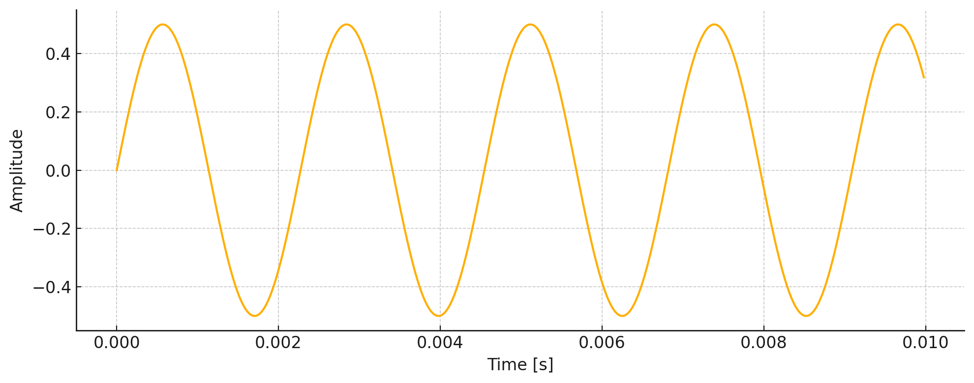
This is a waveform of a 440 Hz wave, plotted over a short duration of 10 milliseconds (ms). This is called a time-domain representation, showing how the wave’s amplitude changes over time. This waveform shows the raw signal as it appears in an audio editor. The ups and downs reflect changes in loudness.
Amplitude
Amplitude is the strength or intensity of a sound wave—in other words, how loud the sound is to the listener. In the previous image, it’s represented by the height of the wave from its center line.
A higher amplitude means a louder sound, while a lower amplitude means a quieter sound. When you adjust the volume on your device, you’re actually changing the amplitude of the audio signal. In digital audio, amplitude is typically measured in decibels (dB) or as a normalized value between -1 and 1.
Frequency
Frequency is how many times a sound wave repeats itself in one second, measured in hertz (Hz). For example, a low bass note is a sound wave that repeats slowly, about 50–100 Hz. In contrast, a high-pitched whistle has a wave that repeats much faster, around 2000–3000 Hz.
In music, different frequencies create different musical notes. For instance, the A4 note that musicians use to tune their instruments is exactly 440 Hz. Now, if you were to look at the frequency plot of the 440 Hz waveform from before, here’s what you’d see:
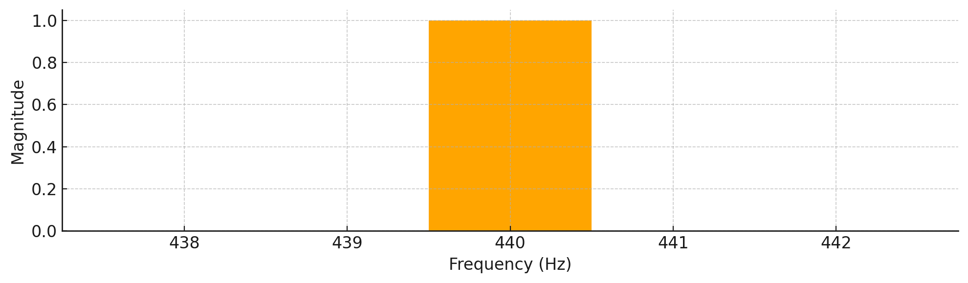
This plot displays the signal in the frequency domain, which shows how much of each frequency is present in the sound. The distinct peak at 440 Hz indicates that this is the dominant frequency in the signal, which is exactly what you’d expect from a pure tone. While time-domain plots—like the one you saw earlier—reveal how the sound’s amplitude changes over time, frequency-domain plots help you understand which frequencies make up the sound.
The waveform you just explored was from a 440 Hz wave. You’ll soon see that many examples in audio processing also deal with this mysterious frequency. So, what makes it so special?
Note: The 440 Hz frequency (A4 note) is the international standard pitch reference for tuning instruments. Its clear, single-frequency nature makes it great for audio tasks. These include sampling, frequency analysis, and waveform representation.
Now that you understand frequency and how it relates to sound waves, you might be wondering how computers actually capture and store these waves.
Sampling
When you record sound digitally, you’re taking snapshots of the audio wave many times per second. Each snapshot measures the wave’s amplitude at that instant. This is called sampling. The number of snapshots taken per second is the sampling rate, measured in hertz (Hz).
When recording digital audio, you need to sample at least twice as fast as the highest frequency you want to capture. This is known as the Nyquist rate. The human ear can hear frequencies up to around 20,000 Hz, which is why audio formats like CDs use a 44,100 Hz sampling rate to accurately capture the full range of human hearing.
Here’s what sampling looks like in practice:

The orange line shows the original continuous sound wave, and the dots show the discrete samples with a sample rate of 20, which means the signal is sampled 20 times per second. These samples are what your computer actually stores and processes. A higher sampling rate lets you reconstruct the original wave more accurately.
Understanding these fundamental concepts, like waveforms, amplitude, frequency, and sampling, is crucial for working with audio data. These ideas are key to audio signal processing. They’ll help you see how TorchAudio manipulates and transforms audio data in a way that machine learning models understand.
Speaking of TorchAudio, now it’s time for you to learn how to install it and explore how it helps with audio data in your machine learning projects.
Get Started With TorchAudio
TorchAudio is a PyTorch-based toolkit for all things audio—from loading and preprocessing data to working with speech, music, and other sound files.
You can transform audio into formats like spectrograms for deep analysis and feed it into your machine learning models. This means you can preprocess your audio data and then train models for tasks like speech recognition, all within the PyTorch framework.
Install TorchAudio
Before performing any audio-related processes, you must install TorchAudio, which extends PyTorch’s capabilities to handle audio data. It uses the same tensor operations, GPU acceleration, and automatic differentiation that PyTorch provides for neural networks, but applies them specifically to audio processing tasks. This means your audio processing pipeline integrates with PyTorch models using consistent data structures and computational methods.
Note: You don’t need to install PyTorch separately, as it’s automatically pulled as a dependency when you install TorchAudio. However, if you’ve already installed PyTorch and would like to continue working in your current Python environment, then you must ensure that the correct pair of torch and torchaudio packages are installed. Check the compatibility matrix on the official website for more details.
To follow along with this tutorial, you’ll need to install TorchAudio and a few additional libraries. You can install them using either Conda or pip, depending on your setup. However, keep in mind that while Conda offers convenient dependency management, its packages may lag slightly behind the latest versions available on PyPI.
Either way, creating a separate virtual environment first is recommended to isolate these dependencies from other projects. If you use Conda, then run the following commands in your terminal:
While numpy, matplotlib, and jupyterlab are core packages available through the defaults channel, it’s best to install torchaudio from the pytorch channel to ensure compatibility with any existing PyTorch installation. Other community-driven packages are typically found in the conda-forge channel.
Note: JupyterLab is a modern, more advanced alternative to the classic Jupyter Notebook. If you prefer working in a browser-based interactive environment, then you can install either of those.
Alternatively, if you’re a pip user, then use these commands instead:
To check whether the installation of TorchAudio worked or not, fire up the Python REPL within your activated virtual environment and run the following code snippet:
>>> import torchaudio

>>> torchaudio.__version__
'2.7.0+cu126'

>>> torchaudio.list_audio_backends()
['soundfile']
If you see a string like '2.5.1' or '2.7.0+cu126' in the output, then you’ve successfully installed TorchAudio. Additionally, you want to ensure at least one of three supported audio backends (ffmpeg, sox, or soundfile) is available so that you can load and save audio data using TorchAudio.
Now that you have TorchAudio properly installed, it’s time to load the dataset you’ll be using throughout the tutorial.
Explore the Speech Commands Dataset
In this tutorial, you’ll work with the Speech Commands dataset. It was created by Pete Warden at Google and released as part of the TensorFlow Speech Recognition Challenge. This dataset includes audio recordings, and it’s meant for training and testing machine learning models in speech recognition tasks.
This dataset includes over 105,000 one-second audio clips. Each clip features one of 35 short words or commands—like “yes,” “no,” “cat,” “up,” “down,” or a number—spoken by a wide range of people. The dataset is designed to help build and evaluate voice-controlled tools, speech recognition systems, and audio processing algorithms.
Load the Dataset Using TorchAudio
To access the Speech Commands dataset, you can take advantage of the SPEECHCOMMANDS class from TorchAudio. It can optionally download and extract a .tar.gz archive with this dataset for you.
Note: The archive is approximately 2.4 GB, and the extracted contents require up to 25 GB of additional disk space. Download and extraction times may vary depending on your internet connection and disk performance.
To get the dataset into your current working directory, you can use Python’s pathlib module together with TorchAudio’s SPEECHCOMMANDS class:
>>> from pathlib import Path
>>> from torchaudio.datasets import SPEECHCOMMANDS
>>> speech_commands_dataset = SPEECHCOMMANDS(root=Path.cwd(), download=True)
By default, this code saves the dataset to your project’s root directory under the SpeechCommands/ subfolder. Note that even with download=True, TorchAudio won’t automatically download the files again if they already exist at the specified location. It’ll instead reuse previously downloaded data.
Take a look at your project directory, which should look something like this:
./
│
└── SpeechCommands/
    │
    └── speech_commands_v0.02/
        │
        ├── backward/
        │   ├── 0165e0e8_nohash_0.wav
        │   ├── 017c4098_nohash_0.wav
        │   └── ...
        │
        ├── bed/
        │   ├── 00176480_nohash_0.wav
        │   ├── 004ae714_nohash_0.wav
        │   └── ...
        │
        ├── bird/
        │   ├── 00970ce1_nohash_0.wav
        │   ├── 00b01445_nohash_0.wav
        │   └── ...
        │
        └── ...
You can access these audio files and their metadata in Python using your speech_commands_dataset variable. The resulting PyTorch dataset object comes with only one public method and supports the square bracket syntax:
>>> speech_commands_dataset.get_metadata(10)
(
    'speech_commands_v0.02/backward/02ade946_nohash_4.wav',
    16000,
    'backward',
    '02ade946',
    4
)

>>> speech_commands_dataset[10]
(
    tensor([[ 0.0000e+00, -9.1553e-05, -3.0518e-05,  ...,  -2.1362e-04]]),
    16000,
    'backward',
    '02ade946',
    4
)
The .get_metadata() method accepts a sample’s numeric index as an argument and returns a Python tuple containing these five elements:
- Relative path to the audio file
- Sample rate
- Label
- Speaker ID
- Utterance number
When you access the same sample using square bracket notation—like speech_commands_dataset[10]—then you’ll get a tuple that mirrors the output of .get_metadata(10), except for the first element. Instead of a file path, you’ll get a PyTorch tensor representing the raw audio waveform. The rest of the tuple remains unchanged.
To make working with such dataset samples more convenient, you can wrap them in equivalent namedtuple instances. Go ahead and create a new Python module—for example, one named speech.py—with the following content:
speech.py
from typing import NamedTuple
from torch import Tensor

class SpeechSample(NamedTuple):
    waveform: Tensor
    sample_rate: int
    label: str
    speaker_id: str
    utterance_number: int
In this helper module, you’ve defined a custom SpeechSample class that extends typing.NamedTuple, giving meaningful names and explicit types to its elements. This design lets you access each part of a dataset sample by name rather than by index, improving code readability and reducing the need to remember the order or meaning of tuple elements.
You’re all set! It’s time to dig into the dataset itself.
Load an Example Audio File
You can now access the audio files in the dataset by picking any index to load. In this tutorial, you’ll stick with a sample at index 10, which corresponds to the word “backward” for the sake of straightforwardness:
>>> from pathlib import Path
>>> from torchaudio.datasets import SPEECHCOMMANDS
>>> from speech import SpeechSample
>>> speech_commands_dataset = SPEECHCOMMANDS(root=Path.cwd(), download=True)
>>> speech_sample = SpeechSample(*speech_commands_dataset[10])
>>> speech_sample
SpeechSample(
    waveform=tensor([[ 0.0000e+00, -9.1553e-05,  ...,  -2.1362e-04]]),
    sample_rate=16000,
    label='backward',
    speaker_id='02ade946',
    utterance_number=4
)
>>> speech_sample.sample_rate
16000
After importing the necessary modules—including your helper speech module—and creating the dataset object, you load a specific audio sample. The conversion from the returned regular tuple to your SpeechSample boils down to unpacking its elements using the star operator (*) and passing them as arguments to the SpeechSample constructor.
You’ll be most interested in processing the following attributes:
| Attribute | Description |
|---|---|
.waveform |
Tensor representing the audio signal |
.sample_rate |
Integer indicating the number of samples per second (Hz) |
.label |
String containing what the voice actor is saying in the audio file |
With the audio sample loaded and its key attributes readily accessible, you’re now ready to dive deeper. Next, you’ll examine the waveform tensor to understand how TorchAudio represents sound, and how you can work with it using PyTorch’s powerful tools.
Understand Audio Tensors (Waveforms)
In TorchAudio, a waveform is a tensor representation of audio data. An audio signal is represented as a PyTorch tensor, which makes it straightforward to manipulate and process using the tools available in PyTorch and TorchAudio.
As you learned earlier, a waveform represents the variation of an audio signal over time. It shows a sound wave graph with the x-axis depicting time, and the y-axis showing the wave’s amplitude. For the speech sample that you just loaded, it looks something like this:

You can get more information about your audio file by checking the shape of your waveform tensor:
>>> speech_sample.waveform.shape
torch.Size([1, 16000])
The first dimension of this tensor is 1, which indicates that the audio file is mono—that is, it contains a single channel of audio data. If the audio file were a stereo file, this dimension would be 2, representing the left and right audio channels.
The second dimension is 16000, which represents the total number of audio samples in the waveform. Each sample corresponds to an amplitude value at a specific point in time.
Since the general shape of a waveform tensor is [channels, samples], you can expose these values through your SpeechSample class. Here’s how you can extend the class by adding two computed properties that provide easy access to the number of channels and the number of samples:
speech.py
from typing import NamedTuple
from torch import Tensor

class SpeechSample(NamedTuple):
    waveform: Tensor
    sample_rate: int
    label: str
    speaker_id: str
    utterance_number: int

    @property
    def num_channels(self) -> int:
        return self.waveform.size(0)

    @property
    def num_samples(self) -> int:
        return self.waveform.size(1)
In both cases, you call the tensor’s .size() method to retrieve the length of the corresponding dimension. When you reimport the updated class, you’ll be able to use its new properties:
>>> speech_sample.num_channels
1

>>> speech_sample.num_samples
16000
In the same way, you can define a convenient property to calculate the sample’s duration in seconds:
speech.py
from typing import NamedTuple
from torch import Tensor

class SpeechSample(NamedTuple):
    # ...

    @property
    def num_seconds(self) -> float:
        return self.num_samples / self.sample_rate
Dividing the total number of samples by the sampling rate yields the audio length in seconds.
Now, you know how to access individual audio files in your dataset and view their tensors. But you can’t really know what’s inside them! How can you actually listen to your audio files?
Listen to Your Audio Files
There are many ways to play sound in Python using third-party libraries. One popular option is sounddevice, which lets you play audio samples directly from a NumPy array. If you’ve been following along, then you should already have both libraries installed in your environment.
To convert a PyTorch tensor into a NumPy array, call .numpy() on it. Remember that you may need to reshape the resulting array so that it reflects the number of audio channels, as sounddevice.play() expects the following data format:
The columns of a two-dimensional array are interpreted as channels, one-dimensional arrays are treated as mono data. (Source)
Given that information, you can implement the following method in your class:
speech.py
from typing import NamedTuple

import sounddevice as sd
from torch import Tensor

class SpeechSample(NamedTuple):
    # ...

    def play(self) -> None:
        sd.play(
            self.waveform.numpy().reshape(-1, self.num_channels),
            self.sample_rate,
            blocking=True
        )
First, you convert the tensor to a NumPy array and reshape it to match the expected format for multi-channel playback. The audio is then played synchronously by setting blocking=True, rather than playing in the background, using the appropriate sample rate.
Alternatively, if you’re working through this tutorial in a Jupyter Notebook, then you can leverage the IPython.display.Audio widget to listen to your audio files interactively:
speech.py
from typing import NamedTuple

import sounddevice as sd
from IPython.display import Audio
from torch import Tensor

class SpeechSample(NamedTuple):
    # ...

    def play_widget(self) -> Audio:
        return Audio(
            self.waveform.numpy(),
            rate=self.sample_rate,
            autoplay=True
        )
The Audio constructor takes a NumPy array obtained from the waveform tensor. It also takes the audio’s sample_rate and an optional autoplay flag, which determines whether the audio should start playing automatically.
When you call your new method in a cell of a Jupyter Notebook, you should see an interactive widget appear and hear an actor saying the word “backward”. This is what the widget looks like:

You can play around with the index parameter and explore other audio files in this dataset. Next, it’s time to prepare your audio dataset for a deep learning model.
Investigate Preprocessing and Data Augmentation Methods
Before feeding audio data into a deep learning model, you’ll need to transform it into a format that the model can understand. This involves standardizing and augmenting your audio signals through techniques like:
- Resampling to adjust sample rates
- Padding and trimming to handle audio lengths
- Adding noise to make your model more robust
You’ll explore each of these preprocessing methods now.
Resample Audio
Resampling changes an audio signal’s sample rate, or the number of audio samples taken per second measured in hertz. For example, a sample rate of 44.1 kilohertz (kHz) means that 44,100 samples are taken every second. You can either increase the sample rate by upsampling, or decrease it by downsampling, depending on your needs.
Note: The 44.1 kHz sample rate captures frequencies up to 22.05 kHz. This is just above the highest frequency that humans can hear, which is 20 kHz. The Nyquist-Shannon sampling theorem requires sampling at twice the highest frequency. Since human hearing ranges from 20 Hz to 20 kHz, a 44.1 kHz sampling rate maintains high-quality audio while keeping file sizes manageable.
You might be asking: Why would you need to resample your audio dataset in the first place? There are a couple of key reasons:
-
Processing Requirements: Some audio processing algorithms or applications require a specific sample rate. Many speech recognition models, like Siri, Google Assistant, and Alexa, are trained on 16 kHz audio.
-
File Size: Lowering the sample rate makes the file smaller. This helps save storage space and cuts down on bandwidth for streaming.
TorchAudio provides a resample() function under the torchaudio.functional module. Here’s how you can incorporate it into your SpeechSample class to resample the underlying audio file:
speech.py
 1from copy import replace
 2from typing import NamedTuple, Self
 3
 4import sounddevice as sd
 5from IPython.display import Audio
 6from torch import Tensor
 7from torchaudio import functional as AF
 8
 9class SpeechSample(NamedTuple):
10    # ...
11
12    def resample(self, sample_rate: int) -> Self:
13        return replace(
14            self,
15            sample_rate=sample_rate,
16            waveform=AF.resample(
17                self.waveform,
18                orig_freq=self.sample_rate,
19                new_freq=sample_rate,
20            )
21        )
There are several elements at play here, so it might help to go through them line by line:
- Line 1 imports the
replace()function from Python’scopymodule, which you’ll use to make shallow copies of your speech samples. Note that this function is only available starting in Python 3.13. If you’re using an earlier version, then check out the workaround below. - Line 2 imports
typing.Selfto annotate methods that returnself. - Line 7 imports the
functionalmodule from TorchAudio and aliases it asAF, allowing you to access itsresample()function to change the sample rate of the audio waveform. - Lines 12 to 21 define the corresponding
.resample()wrapper method within your class. This method takes the desired sample rate as an argument and returns a newSpeechSampleobject with the waveform resampled to the specified rate. - Line 13 calls
replace()to create a new instance ofSpeechSamplewith the updated sample rate and waveform, ensuring the original instance remains unchanged.
If you’re working with an older version of Python that doesn’t support copy.replace(), then you can define a fallback to replicate similar behavior. Add the following snippet at the top of your Python module:
speech.py
try:
    from copy import replace
except ImportError:
    def replace(obj, **kwargs):
        return obj._replace(**kwargs)

# ...
You leverage the ._replace() method available on named tuples to mimic the functionality of copy.replace(). While it works for simple use cases involving named tuples, it lacks the flexibility and safety of the newer function. Use it cautiously, and only as a temporary measure when upgrading Python isn’t an option.
When you reload the Python REPL or restart your Jupyter Notebook, you’ll be able to hear the difference between the original speech sample and a resampled one:
>>> speech_sample = SpeechSample(*speech_commands_dataset[10])
>>> speech_sample.play()

>>> resampled_audio = speech_sample.resample(sample_rate=4000)
>>> resampled_audio.play()
The quality has slightly dropped, but you can clearly understand what the actor is saying.
Now that you understand how to adjust sample rates, how do you handle audio clips of different lengths in your dataset? It’s time to explore padding and trimming techniques to standardize your audio durations.
Apply Padding and Trimming
Padding and trimming audio files are common preprocessing steps. They help ensure all the audio samples in your dataset are the same length:
- Padding: Adds extra data, often zeros, to the start or end of an audio signal. This makes the signal longer and meets a specific size requirement.
- Trimming: Involves cutting off parts of an audio signal to reduce its length to a specific size. Most neural networks require a fixed input size, and padding and trimming make sure that all audio samples meet this requirement.
PyTorch’s torch.nn.functional offers the pad() function that you can use for padding your audio files. To trim audio in Python, just use sequence slicing. This lets you cut parts of the audio signal and make it a specific length:
speech.py
from copy import replace
from typing import NamedTuple

import sounddevice as sd
from IPython.display import Audio
from torch import Tensor
from torch.nn import functional as F
from torchaudio import functional as AF

class SpeechSample(NamedTuple):
    # ...

    def pad_trim(self, seconds: int | float) -> Self:
        num_samples = int(self.sample_rate * seconds)
        if self.num_samples > num_samples:
            return replace(self, waveform=self.waveform[:, :num_samples])
        elif self.num_samples < num_samples:
            padding_amount = num_samples - self.num_samples
            return replace(
                self, waveform=F.pad(self.waveform, (0, padding_amount))
            )
        else:
            return self
The .pad_trim() method makes sure that your waveform is padded or trimmed to exactly the given number of seconds along the second dimension. In it, you calculate the required number of samples using the sampling rate. If the waveform is longer than the specified duration, then you truncate it. If it’s shorter, then you pad it with zeros at the end. Otherwise, you return the original speech sample.
Most of the audio files in the Speech Commands dataset are one second long, but some are slightly longer or shorter. To make sure all data is uniform without losing any information, you can use .pad_trim() with two seconds as the target length:
>>> fixed_length_audio = speech_sample.pad_trim(seconds=2)
>>> fixed_length_audio.num_samples
32000
>>> fixed_length_audio.sample_rate
16000
>>> fixed_length_audio.num_seconds
2.0
Here, you’re making sure that your audio waveform is exactly two seconds long by padding or trimming the original waveform as needed. The final waveform has a fixed length of 32,000 samples at a 16,000 Hz sampling rate.
Warning: Don’t confuse torch.nn.functional with torchaudio.functional:
torchaudio.functionalprovides audio-specific operations, such as resampling and other signal processing utilities.torch.nn.functionalcontains general-purpose tensor operations, like padding, which apply to a wide range of data types, including audio, images, and more.
Be sure to use each module appropriately based on the context of your task.
Your .pad_trim() method works as intended, but you’ve only applied it to one audio file so far. In the next step, you’ll use it alongside other preprocessing methods to prepare every audio file in your dataset for training.
Standardize the Dataset
Before moving on, define another helper method in your SpeechSample class that will let you save the preprocessed audio sample to disk at the specified file path:
speech.py
from copy import replace
from pathlib import Path
from typing import NamedTuple, Self

import sounddevice as sd
import torchaudio
from IPython.display import Audio
from torch import Tensor
from torch.nn import functional as F
from torchaudio import functional as AF

class SpeechSample(NamedTuple):
    # ...

    def save(self, path: str | Path) -> None:
        torchaudio.save(path, self.waveform, self.sample_rate)
Under the hood, this method delegates the actual work to torchaudio.save(), supplying it with the file path, waveform tensor, and sample rate. By wrapping this call within a method of your SpeechSample class, you provide a streamlined interface for saving audio data. This ensures that the audio is saved consistently with the correct parameters, reducing the likelihood of errors.
Next, you’ll define a module-level function in your speech.py file to handle the bulk processing logic for the Speech Commands dataset:
speech.py
 1from copy import replace
 2from pathlib import Path
 3from typing import NamedTuple, Self
 4
 5import sounddevice as sd
 6import torchaudio
 7from IPython.display import Audio
 8from torch import Tensor
 9from torch.nn import functional as F
10from torchaudio import functional as AF
11from torchaudio.datasets import SPEECHCOMMANDS
12from tqdm import tqdm
13
14# ...
15
16def bulk_process(
17    dataset: SPEECHCOMMANDS,
18    output_dir: str | Path,
19    sample_rate: int,
20    seconds: int | float,
21) -> None:
22    for index, sample in tqdm(enumerate(dataset), total=len(dataset)):
23        speech_sample = SpeechSample(*sample)
24        input_path, *_ = dataset.get_metadata(index)
25        output_path = Path(output_dir).resolve() / input_path
26        output_path.parent.mkdir(parents=True, exist_ok=True)
27        if speech_sample.sample_rate != sample_rate:
28            speech_sample = speech_sample.resample(sample_rate)
29        speech_sample = speech_sample.pad_trim(seconds)
30        speech_sample.save(output_path)
Here’s a line-by-line breakdown:
- Lines 11 and 12 import
SPEECHCOMMANDSfor type hinting andtqdmfor displaying a progress bar, respectively. - Lines 16 to 30 define the
bulk_process()function, which iterates over the dataset, processes each audio file by resampling and trimming it to the desired duration, and saves the processed audio to the specified output directory. - Line 22 runs a
forloop over dataset samples and their indices usingenumerate(). The loop counter is wrapped with a call totqdm(), which adds a progress bar to visually track the loop’s execution. - Line 23 creates a
SpeechSampleinstance by unpacking the raw tuple from TorchAudio. - Line 24 retrieves metadata about the current sample. It destructures the first element as
input_pathand discards the rest using*_. This yields the original file path relative to the dataset root folder. - Lines 25 and 26 determine the output file’s destination and recursively create any missing parent folders, suppressing errors if the directories already exist.
- Lines 27 to 29 optionally resample the audio and pad or trim it to match the given parameters, ensuring all processed files have a uniform format and exact length.
- Line 30 saves the processed sample to
output_pathusing the.save()method you defined earlier, writing the waveform to disk.
You can now return to the Python REPL, load the Speech Commands dataset, and bulk process it with your new function:
>>> from pathlib import Path
>>> from torchaudio.datasets import SPEECHCOMMANDS
>>> from speech import bulk_process
>>> bulk_process(
...     SPEECHCOMMANDS(root=Path.cwd(), download=True),
...     output_dir=Path("SpeechCommandsProcessed"),
...     sample_rate=16000,
...     seconds=2,
... )
 23%|██████████                      | 23864/105829 [08:11<26:04, 52.38it/s]
This code applies your desired standardization across your entire dataset. Please note that processing all 105,000+ words may take several minutes. The progress bar will update in real-time to show the current status of the operation.
When done, the SpeechCommandsProcessed/ directory will mirror the structure and content of the original SpeechCommands/, with both sitting at the root of your project:
./
│
├── SpeechCommands/
│   │
│   └── (...)
│
└── SpeechCommandsProcessed/
    │
    └── speech_commands_v0.02/
        │
        ├── backward/
        │   ├── 0165e0e8_nohash_0.wav
        │   ├── 017c4098_nohash_0.wav
        │   └── ...
        │
        ├── bed/
        │   ├── 00176480_nohash_0.wav
        │   ├── 004ae714_nohash_0.wav
        │   └── ...
        │
        ├── bird/
        │   ├── 00970ce1_nohash_0.wav
        │   ├── 00b01445_nohash_0.wav
        │   └── ...
        │
        └── ...
As long as you haven’t changed the original 16 kHz sampling rate, you can load your processed dataset by explicitly setting the folder_in_archive parameter in the SPEECHCOMMANDS call:
>>> from pathlib import Path
>>> from torchaudio.datasets import SPEECHCOMMANDS
>>> from speech import SpeechSample
>>> processed_dataset = SPEECHCOMMANDS(
...     root=Path.cwd(),
...     folder_in_archive="SpeechCommandsProcessed"
... )
>>> speech_sample = SpeechSample(*processed_dataset[10])
>>> speech_sample.num_seconds
2.0
However, since TorchAudio hard-codes a 16 kHz sample rate in its source code, you’ll need to create a custom dataset if you want to resample the audio. You’ll explore how to do that later.
The bulk_process() function makes sure all your audio files are the same length—a key step for working with audio data. Next up, you’ll look at how to handle another common issue: differences in audio volume across your dataset.
Normalize Audio
The recordings in the Speech Commands dataset come from various speakers, environments, and devices, leading to variations in amplitude across different samples. This inconsistency can cause problems for your machine learning model, as it might make the model overly sensitive to the volume of the dataset rather than focusing on more useful characteristics of the audio files.
To avoid this problem, it’s best to normalize your dataset. This means adjusting the amplitude values of all your audio signals to a specific range or standard. Fortunately, the torchaudio.load() function, which is used behind the scenes, offers a normalize parameter, which is set to True by default. So, TorchAudio has you covered, and you don’t need to take any extra steps!
Note: Keep in mind that torchaudio.load() normalizes the waveform amplitude, scaling the sampled values to fall within the range of [-1.0, 1.0]. While this normalization ensures consistency in data representation across different audio formats, it doesn’t change the perceived loudness or volume of your audio files. To adjust the loudness, use techniques like LUFS (Loudness Units relative to Full Scale).
So far, you’ve standardized your audio files and made sure they have consistent volume levels. But how can you transform your audio data in a more intuitive way to visualize it?
Create Spectrograms
To get a machine learning model to understand audio, you often need to move from the time domain to the frequency domain. You need a numerical presentation of your audio file that tells you which parts of the sound contain which notes or tones, and at what time. A spectrogram helps you do exactly that:
A spectrogram is a visual representation of the spectrum of frequencies of a signal as it varies with time. When applied to an audio signal, spectrograms are sometimes called sonographs, voiceprints, or voicegrams. (Source)
To create a spectrogram, you need to perform a Fourier transform (FT) on small segments of the audio signal. The Fast Fourier Transform (FFT) is the algorithm used for this, and it requires you to specify the number of frequency points you want to compute.
Here’s how the spectrogram transformation works:
- The audio signal is divided into small, overlapping segments called windows that are typically a few milliseconds long.
- For each window, the FFT analyzes which frequencies are present and how strong they are.
- The windows overlap and slide along the audio signal, creating a series of frequency snapshots.
- These snapshots are combined to form the spectrogram, showing how frequencies change over time.
This technique is called Short-Time Fourier Transform (STFT) because it analyzes short segments of audio rather than processing the entire signal at once. The short-time approach allows you to see how frequencies evolve throughout your audio clip. The result is a detailed picture showing how the frequencies in your audio change from moment to moment, which is exactly what a spectrogram displays.
Note: If you want to get hands-on with Fourier transforms in Python, then check out Fourier Transforms With scipy.fft: Python Signal Processing to learn how to apply them directly in your projects.
Now that you know how spectrograms are made, it’s time to make one. To create a spectrogram in TorchAudio, you’ll use the Spectrogram class from torchaudio.transforms:
>>> import torchaudio.transforms as T
>>> spectrogram_transform = T.Spectrogram(
...     n_fft=1024,
...     win_length=None,
...     hop_length=512,
...     normalized=True
... )
When creating a spectrogram, you need to specify a few parameters:
| Parameter | Meaning | Effect on Spectrogram |
|---|---|---|
n_fft |
Number of samples per FFT | Higher values give better frequency resolution (more frequency bins) |
win_length |
Length of each window in samples | If None, defaults to n_fft |
hop_length |
Number of samples between successive windows | Smaller values give better time resolution (more overlap) |
You can feed your audio file to the spectrogram_transform you created earlier to see what your spectrogram looks like so far:
>>> spectrogram = spectrogram_transform(speech_sample.waveform)
>>> spectrogram
tensor([[[4.0992e-08, 1.2626e-10, 5.0785e-08,  ..., 2.1378e-08,
          1.1199e-08, 1.1576e-09],
         [1.3024e-07, 2.1598e-08, 1.2256e-07,  ..., 1.0029e-07,
          7.8936e-09, 4.8156e-08],
         [1.8714e-07, 1.3087e-07, 4.9596e-08,  ..., 4.7979e-07,
          1.7561e-07, 1.6183e-07],
         ...,
         [3.4479e-10, 3.5584e-10, 7.7859e-12,  ..., 2.4817e-10,
          6.2482e-12, 4.3299e-10],
         [2.4906e-09, 3.5388e-10, 3.8308e-11,  ..., 9.0459e-11,
          3.4527e-10, 4.4065e-10],
         [4.6073e-09, 7.3008e-10, 6.5713e-11,  ..., 5.0754e-11,
          4.5115e-10, 1.7723e-09]]])
>>> spectrogram.shape
torch.Size([1, 513, 32])
The values inside the tensor are the magnitudes of the frequency components at each time frame. As you can see from the output, the spectrogram tensor has three dimensions:
| Dimension | Description |
|---|---|
| Channels | Number of separate audio signals in the input |
| Frequency Bins | Number of frequency components analyzed in each time segment |
| Time Steps | Number of time segments the audio is divided into for analysis |
So, for your audio file above, it tells you that it has one channel, 513 frequency bins, and that the audio was split into 32 small overlapping chunks for analysis.
You can visualize your spectrogram to get a more intuitive understanding. To do this, you can create a two-dimensional plot, where:
- The x-axis represents time.
- The y-axis represents frequency.
- The color intensity represents the magnitude, with brighter colors indicating higher energy.
Before you jump into that, you need to apply a transformation to your spectrogram tensor. The raw values in a spectrogram represent power or magnitude. They show how strong each frequency is at each moment in time. But these values are often very small and can span a wide range, making it hard to interpret or visualize them directly. That’s where the decibel (dB) scale comes in.
The decibel scale:
- Compresses a large range of values into a more readable scale
- Emphasizes differences between loud and quiet parts
- Matches human perception more closely—your ears perceive loudness logarithmically, not linearly
TorchAudio gives you a straightforward way to do this. You can import AmplitudeToDB from torchaudio.transforms and apply it to your spectrogram:
>>> from torchaudio.transforms import AmplitudeToDB
>>> spectrogram_db = T.AmplitudeToDB()(spectrogram)
>>> spectrogram_db
tensor([[[ -73.8730,  -98.9874,  -72.9426,  ...,  -76.7003,  -79.5084,
           -89.3645],
         [ -68.8526,  -76.6559,  -69.1164,  ...,  -69.9872,  -81.0273,
           -73.1735],
         [ -67.2783,  -68.8316,  -73.0456,  ...,  -63.1895,  -67.5546,
           -67.9095],
         ...,
         [ -94.6244,  -94.4875, -100.0000,  ...,  -96.0526, -100.0000,
           -93.6352],
         [ -86.0369,  -94.5114, -100.0000,  ..., -100.0000,  -94.6185,
           -93.5591],
         [ -83.3656,  -91.3663, -100.0000,  ..., -100.0000,  -93.4568,
           -87.5146]]])
The conversion to decibels transforms your raw spectrogram values into a more interpretable scale, with values typically ranging from -100 dB (very quiet) to 0 dB (maximum intensity).
Visualize Audio Spectrograms
To plot all of this information and visualize your audio file’s spectrogram, you can use Matplotlib:
>>> import matplotlib.pyplot as plt
>>> plt.figure(figsize=(15, 8))
<Figure size 1500x800 with 0 Axes>
>>> plt.subplot(2, 1, 1)
<Axes: >
>>> plt.imshow(
...     spectrogram_db[0].numpy(),
...     aspect="auto",
...     origin="lower",
...     cmap="magma",
...     extent=[
...         0, speech_sample.num_seconds,
...         0, spectrogram_transform.n_fft // 2
...     ]
... )
<matplotlib.image.AxesImage object at 0x7585d54d9a90>
>>> plt.colorbar(format="%+2.0f dB")
<matplotlib.colorbar.Colorbar object at 0x7585d4e86a50>
>>> plt.title(f"Spectrogram - Label: {speech_sample.label}")
Text(0.5, 1.0, 'Spectrogram - Label: backward')
>>> plt.ylabel("Frequency (Hz)")
Text(0, 0.5, 'Frequency (Hz)')
>>> plt.tight_layout()
>>> plt.show()
You’re plotting frequency on the y-axis, time on the x-axis, and using color to show the intensity of each frequency over time.
Here’s what your spectrogram looks like:

The vertical shapes show when the speaker is producing sound. These are bursts of energy during speech. The horizontal bands inside each burst show which frequencies are active. These patterns are especially important in speech and can help your model distinguish between different words. The dark areas indicate silence or low-energy parts of the waveform. You can try visualizing other audio files to see how their patterns differ.
To apply such transforms to your SpeechSample objects, you can define the appropriate wrapper method:
speech.py
from copy import replace
from pathlib import Path
from typing import Callable, NamedTuple, Self

import sounddevice as sd
import torchaudio
from IPython.display import Audio
from torch import Tensor
from torch.nn import functional as F
from torchaudio import functional as AF
from torchaudio.datasets import SPEECHCOMMANDS
from tqdm import tqdm

class SpeechSample(NamedTuple):
    # ...

    def apply(self, transform: Callable[[Tensor], Tensor]) -> Self:
        return replace(self, waveform=transform(self.waveform))

# ...
It returns a copy of the original speech sample with the transformed waveform tensor.
While spectrograms give you a clear visual representation of your audio data, what happens when that data contains unwanted noise or interference? This leads to another important preprocessing technique: adding controlled noise to make your model more robust.
Add Additive White Gaussian Noise (AWGN)
To improve your machine learning model’s ability to generalize, adding noise to your data is often necessary. This might sound strange at first, but there are good reasons for doing it.
Note: When you add noise to your data in machine learning, it means you intentionally introduce some random variations or small errors into your dataset.
Adding noise can help make your model more robust and better at generalizing to new, unseen data. It prevents the model from overfitting, which happens when the model learns the details and noise of the training data too well, making it less effective on new data.
One popular method is Additive White Gaussian Noise (AWGN), which simulates real-world randomness by adding a specific type of noise to the signal.
Note: AWGN is additive because it’s added to the original signal. It’s white as it affects all frequencies equally, with constant power spectral density. The term Gaussian refers to its amplitude distribution, which follows a normal (bell-curved) probability density function.
AWGN makes models more robust during training. Adding controlled noise prevents the models from memorizing exact patterns in clean audio. Instead, models learn important features that distinguish sounds, even with interference. Plus, you don’t need to collect new samples or labels—you can create variations by adding different noise levels.
To add AWGN to a waveform, you can create another method in your SpeechSample class. It’ll use PyTorch’s specialized tensor methods to introduce Gaussian noise to your waveform tensors:
speech.py
from copy import replace
from pathlib import Path
from typing import Callable, NamedTuple, Self

import sounddevice as sd
import torchaudio
from IPython.display import Audio
from torch import Tensor, clamp, randn_like
from torch.nn import functional as F
from torchaudio import functional as AF
from torchaudio.datasets import SPEECHCOMMANDS
from tqdm import tqdm

class SpeechSample(NamedTuple):
    # ...

    def with_gaussian_noise(self, level=0.01) -> Self:
        noise = randn_like(self.waveform) * level
        return replace(self, waveform=clamp(self.waveform + noise, -1.0, 1.0))

# ...
Here’s what’s happening in this code:
- First,
randn_like()creates a noise tensor that matches the shape of your waveform. This noise follows a Gaussian distribution centered at0with a standard deviation of1. - The noise is then scaled by
level. A smaller value like0.001creates subtle noise, while a larger value like0.1creates more noticeable interference. - This scaled noise is added directly to your waveform with a good old addition operation (
+). clamp()keeps all values between-1.0and1.0, which is the standard range for audio signals. This prevents distortion in the final audio.
This process creates a controlled amount of interference that can help make your model more robust during training. When you listen to your noisy audio, you’ll notice that the sound is less clear:
>>> noisy_waveform = speech_sample.with_gaussian_noise(0.005)
>>> noisy_waveform.save("noisy_audio.wav")
>>> noisy_waveform.play()
Feel free to experiment with the noise level and observe how it affects the audio quality.
Create a Custom PyTorch Dataset
You now understand the basic data processing steps needed for an audio dataset and how to implement them. However, you had to apply many transformations manually and repeatedly across your entire dataset. PyTorch allows you to handle this more efficiently with custom datasets by extending the Dataset base class.
The two mandatory methods that you must implement in your custom dataset are:
-
.__len__(self): This method returns the total number of items in the dataset. This is important for PyTorch’sDataLoaderto know how many samples to iterate over. -
.__getitem__(self, index): This method retrieves a single item from the dataset based on the given index. This is where you define the logic for loading and processing each data sample individually.
Additionally, while not strictly required, you’ll often specify an .__init__(self) method, where you can set up any attributes, parameters, or preprocessing steps that are needed across all items in the dataset.
Note: In PyTorch, a DataLoader is a built-in class that loads data into a model for training. It’s especially useful for managing large datasets that can’t fit into memory, and for applying data augmentation and preprocessing. To use a DataLoader, you first need to define a concrete subclass of Dataset.
You already have all the necessary logic for preprocessing your data. Now, you can put it all together into a custom dataset. Start by adding a new class, AugmentedSpeechCommands, into your speech module, which will take five input parameters:
speech.py
from copy import replace
from pathlib import Path
from typing import Callable, NamedTuple, Self

import sounddevice as sd
import torchaudio
from IPython.display import Audio
from torch import Tensor, clamp, randn_like
from torch.nn import functional as F
from torch.utils.data import Dataset
from torchaudio import functional as AF
from torchaudio.datasets import SPEECHCOMMANDS
from torchaudio.datasets.speechcommands import FOLDER_IN_ARCHIVE
from tqdm import tqdm

# ...

class AugmentedSpeechCommands(Dataset):
    def __init__(
        self,
        folder: str | Path | None = None,
        seconds: int | float | None = None,
        noise_level: float = 0.005,
        enable_noise: bool = True,
        transform: Callable[[Tensor], Tensor] | None = None
    ) -> None:
        if folder:
            self.folder = Path(folder).resolve()
        else:
            self.folder = Path.cwd() / FOLDER_IN_ARCHIVE
        self._raw_dataset = SPEECHCOMMANDS(
            self.folder.parent,
            folder_in_archive=self.folder.name
        )
        self._noise = noise_level
        self._enable_noise = enable_noise
        self._transform = transform
        self._seconds = seconds

# ...
Your class is a custom PyTorch dataset that loads the Speech Commands audio dataset and provides optional data augmentation. It can inject background noise into the audio and apply custom transformations to help train more robust models. You can set how much noise to add, whether to use noise at all, and how long each audio clip should be. If no folder is given, then it uses the default dataset path from TorchAudio.
Although your class extends PyTorch’s Dataset, you still need to provide your own implementation for the two special methods mentioned earlier:
speech.py
# ...

class AugmentedSpeechCommands(Dataset):
    # ...

    def __len__(self) -> int:
        return len(self._raw_dataset)

    def __getitem__(self, index: int) -> SpeechSample:
        relative_path, _, *metadata = self._raw_dataset.get_metadata(index)
        absolute_path = self.folder / relative_path
        waveform, sample_rate = torchaudio.load(absolute_path)
        speech_sample = SpeechSample(waveform, sample_rate, *metadata)

        if self._seconds is not None:
            speech_sample = speech_sample.pad_trim(self._seconds)

        if self._enable_noise:
            speech_sample = speech_sample.with_gaussian_noise(self._noise)

        if self._transform:
            speech_sample = speech_sample.apply(self._transform)

        return speech_sample

# ...
The first method, .__len__(), returns the number of samples in the dataset. The second method, .__getitem__(), returns the specific sample at the given index. Notice that this method returns your SpeechSample instance, which has meaningful attribute names, rather than a plain tuple. Additionally, your custom dataset applies optional processing to each sample.
Note: You could improve this code by adding a caching layer on top of it. This can optimize performance at the cost of increased memory usage.
To give your custom dataset a spin, you might want to try the following:
>>> from torchaudio import transforms as T
>>> from speech import AugmentedSpeechCommands
>>> custom_dataset = AugmentedSpeechCommands(
...     folder="SpeechCommandsProcessed",
...     seconds=2,
...     noise_level=0.005,
...     enable_noise=True,
...     transform=T.Vol(gain=0.5, gain_type="amplitude")
... )
>>> custom_dataset[10]
SpeechSample(
    waveform=tensor([[-0.0010,  0.0024,  0.0020,  ...,  -0.0016]]),
    sample_rate=4000,
    label='backward',
    speaker_id='02ade946',
    utterance_number=4
)
Now, you have a clean class dedicated to all the transformations you need to train a machine learning model. This Dataset object is a specialized PyTorch object that can be integrated with data loaders, allowing you to take full advantage of PyTorch and TorchAudio’s built-in methods for training audio models.
Next Steps
TorchAudio offers built-in audio deep learning models. You have a PyTorch Dataset object, so you can feed your dataset to these models directly. Here are two built-in deep learning models in TorchAudio:
- Wav2Vec 2.0: A powerful model for speech recognition that uses self-supervised learning on raw audio waveforms. You can fine-tune this model for specific speech recognition tasks.
- DeepSpeech: An end-to-end speech recognition model based on recurrent neural networks (RNNs). It converts audio waveforms directly into text by processing sequences of audio frames.
These models save you from building everything from scratch, so you can focus on preparing your data and fine-tuning the model for your task. TorchAudio makes it easier to build strong speech recognition systems quickly.
Conclusion
Great job! You’ve successfully explored how to harness the power of TorchAudio, effectively processing audio data for your machine learning projects. With these skills, you can now prepare audio data for machine learning tasks like speech recognition, and use it with TorchAudio’s advanced models like Wav2Vec 2.0 and DeepSpeech.
In this tutorial, you’ve learned how to:
- Load and explore audio data using TorchAudio’s Speech Commands dataset
- Standardize audio lengths by padding and trimming waveform tensors
- Transform waveforms into spectrograms for frequency-based insights
- Augment data by adding controlled noise to enhance model robustness
- Create a custom dataset that seamlessly integrates with PyTorch
Keep experimenting with different preprocessing combinations, and don’t hesitate to adapt these techniques to your specific audio challenges. Stay awesome!
Frequently Asked Questions
Now that you have some experience using TorchAudio in Python, you can use the questions and answers below to check your understanding and recap what you’ve learned.
These FAQs are related to the most important concepts you’ve covered in this tutorial. Click the Show/Hide toggle beside each question to reveal the answer.
You use TorchAudio to process audio data for deep learning applications, such as loading datasets, transforming waveforms into spectrograms, and augmenting data with noise.
You load audio data in TorchAudio using the torchaudio.load() function, which reads the audio file and returns a waveform tensor and the sample rate.
TorchAudio normalizes audio by default when you load it using torchaudio.load(), which scales the waveform’s amplitude to fall within the range of -1.0 to 1.0.
You use a spectrogram to visually represent the spectrum of frequencies in an audio signal over time, helping you analyze and understand the frequency components of the sound.
In TorchAudio, you pad audio using PyTorch’s torch.nn.functional.pad(), and trim it using Python’s sequence slicing to ensure that all samples have a uniform length.
Take the Quiz: Test your knowledge with our interactive “Use TorchAudio to Prepare Audio Data for Deep Learning” quiz. You’ll receive a score upon completion to help you track your learning progress:
Interactive Quiz
Use TorchAudio to Prepare Audio Data for Deep LearningTest your grasp of audio fundamentals and working with TorchAudio in Python! You'll cover loading audio datasets, transforms, and more.