There’s an abundance of third-party tools and libraries for manipulating and analyzing audio WAV files in Python. At the same time, the language ships with the little-known wave module in its standard library, offering a quick and straightforward way to read and write such files. Knowing Python’s wave module can help you dip your toes into digital audio processing.
If topics like audio analysis, sound editing, or music synthesis get you excited, then you’re in for a treat, as you’re about to get a taste of them!
In this tutorial, you’ll learn how to:
- Read and write WAV files using pure Python
- Handle the 24-bit PCM encoding of audio samples
- Interpret and plot the underlying amplitude levels
- Record online audio streams like Internet radio stations
- Animate visualizations in the time and frequency domains
- Synthesize sounds and apply special effects
Although not required, you’ll get the most out of this tutorial if you’re familiar with NumPy and Matplotlib, which greatly simplify working with audio data. Additionally, knowing about numeric arrays in Python will help you better understand the underlying data representation in computer memory.
Click the link below to access the bonus materials, where you’ll find sample audio files for practice, as well as the complete source code of all the examples demonstrated in this tutorial:
Get Your Code: Click here to download the free sample code that shows you how to read and write WAV files in Python.
You can also take the quiz to test your knowledge and see how much you’ve learned:
Take the Quiz: Test your knowledge with our interactive “Reading and Writing WAV Files in Python” quiz. You’ll receive a score upon completion to help you track your learning progress:

Interactive Quiz
Reading and Writing WAV Files in PythonIn this quiz, you can test your knowledge of handling WAV audio files in Python with the wave module. By applying what you've learned, you'll demonstrate your ability to synthesize sounds, analyze and visualize waveforms, create dynamic spectrograms, and enhance audio with special effects.
Understand the WAV File Format
In the early nineties, Microsoft and IBM jointly developed the Waveform Audio File Format, often abbreviated as WAVE or WAV, which stems from the file’s extension (.wav). Despite its older age in computer terms, the format remains relevant today. There are several good reasons for its wide adoption, including:
- Simplicity: The WAV file format has a straightforward structure, making it relatively uncomplicated to decode in software and understand by humans.
- Portability: Many software systems and hardware platforms support the WAV file format as standard, making it suitable for data exchange.
- High Fidelity: Because most WAV files contain raw, uncompressed audio data, they’re perfect for applications that require the highest possible sound quality, such as with music production or audio editing. On the flipside, WAV files take up significant storage space compared to lossy compression formats like MP3.
It’s worth noting that WAV files are specialized kinds of the Resource Interchange File Format (RIFF), which is a container format for audio and video streams. Other popular file formats based on RIFF include AVI and MIDI. RIFF itself is an extension of an even older IFF format originally developed by Electronic Arts to store video game resources.
Before diving in, you’ll deconstruct the WAV file format itself to better understand its structure and how it represents sounds. Feel free to jump ahead if you just want to see how to use the wave module in Python.
The Waveform Part of WAV
What you perceive as sound is a disturbance of pressure traveling through a physical medium, such as air or water. At the most fundamental level, every sound is a wave that you can describe using three attributes:
- Amplitude is the measure of the sound wave’s strength, which you perceive as loudness.
- Frequency is the reciprocal of the wavelength or the number of oscillations per second, which corresponds to the pitch.
- Phase is the point in the wave cycle at which the wave starts, not registered by the human ear directly.
The word waveform, which appears in the WAV file format’s name, refers to the graphical depiction of the audio signal’s shape. If you’ve ever opened a sound file using audio editing software, such as Audacity, then you’ve likely seen a visualization of the file’s content that looked something like this:
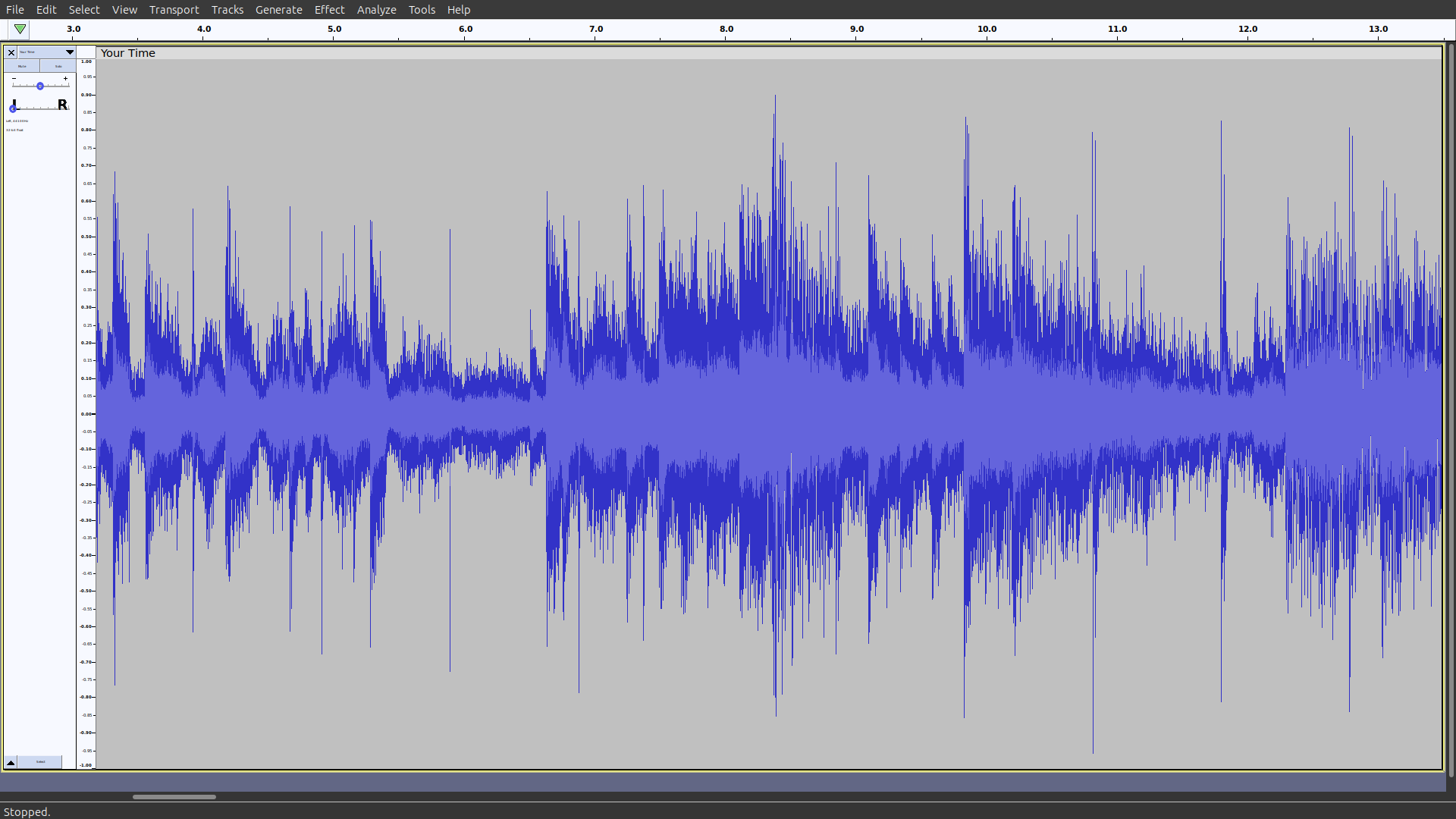
That’s your audio waveform, illustrating how the amplitude changes over time.
The vertical axis represents the amplitude at any given point in time. The midpoint of the graph, which is a horizontal line passing through the center, represents the baseline amplitude or the point of silence. Any deviation from this equilibrium corresponds to a higher positive or negative amplitude, which you experience as a louder sound.
As you move from left to right along the graph’s horizontal scale, which is the timeline, you’re essentially moving forward in time through your audio track.
Having such a view can help you visually inspect the characteristics of your audio file. The series of the amplitude’s peaks and valleys reflect the volume changes. Therefore, you can leverage the waveform to identify parts where certain sounds occur or find quiet sections that may need editing.
Coming up next, you’ll learn how WAV files store these amplitude levels in digital form.
The Structure of a WAV File
The WAV audio file format is a binary format that exhibits the following structure on disk:
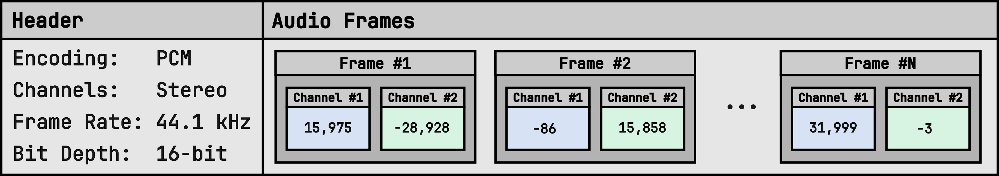
As you can see, a WAV file begins with a header comprised of metadata, which describes how to interpret the sequence of audio frames that follow. Each frame consists of channels that correspond to loudspeakers, such as left and right or front and rear. In turn, every channel contains an encoded audio sample, which is a numeric value representing the relative amplitude level at a given point in time.
The most important parameters that you’ll find in a WAV header are:
- Encoding: The digital representation of a sampled audio signal. Available encoding types include uncompressed linear Pulse-Code Modulation (PCM) and a few compressed formats like ADPCM, A-Law, or μ-Law.
- Channels: The number of channels in each frame, which is usually equal to one for mono and two for stereo audio tracks, but could be more for surround sound recordings.
- Frame Rate: The number of frames per second, also known as the sampling rate or the sampling frequency measured in hertz. It affects the range of representable frequencies, which has an impact on the perceived sound quality.
- Bit Depth: The number of bits per audio sample, which determines the maximum number of distinctive amplitude levels. The higher the bit depth, the greater the dynamic range of the encoded signal, making subtle nuances in the sound audible.
Python’s wave module supports only the Pulse-Code Modulation (PCM) encoding, which is by far the most popular, meaning that you can usually ignore other formats. Moreover, Python is limited to integer data types, while PCM doesn’t stop there, defining several bit depths to choose from, including floating-point ones:
| Data Type | Signed | Bits | Min Value | Max Value |
|---|---|---|---|---|
| Integer | No | 8 | 0 | 255 |
| Integer | Yes | 16 | -32,768 | 32,767 |
| Integer | Yes | 24 | -8,388,608 | 8,388,607 |
| Integer | Yes | 32 | -2,147,483,648 | 2,147,483,647 |
| Floating-Point | Yes | 32 | ≈ -3.40282 × 1038 | ≈ 3.40282 × 1038 |
| Floating-Point | Yes | 64 | ≈ -1.79769 × 10308 | ≈ 1.79769 × 10308 |
In practice, the floating-point data types are overkill for most uses, as they require more storage while providing little return on investment. You probably won’t miss them unless you need extra dynamic range for truly professional sound editing.
Note: Despite dealing with an integer flavor of the PCM encoding, you’ll often want to represent the underlying audio samples as floating-point numbers internally in your source code. This will let you handle various bit depths uniformly and streamline the math behind audio processing.
After reading an audio sample into Python, you’ll typically normalize its value so that it always falls between -1.0 and 1.0 on the scale, regardless of the original range of PCM values. Then, before writing it back to a WAV file, you’ll convert and clamp the value to make it fit the desired range.
The 8-bit integer encoding is the only one relying on unsigned numbers. In contrast, all remaining data types allow both positive and negative sample values.
Another important detail you should take into account when reading audio samples is the byte order. The WAV file format specifies that multi-byte values are stored in little-endian or start with the least significant byte first. Fortunately, you don’t typically need to worry about it when you use the wave module to read or write audio data in Python. Still, there might be edge cases when you do!
The 8-bit, 16-bit, and 32-bit integers have standard representations in the C programming language, which the default CPython interpreter builds on. However, the 24-bit integer is an outlier without a corresponding built-in C data type. Exotic bit depths like that aren’t unheard of in music production, as they help strike a balance between size and quality. Later, you’ll learn how to emulate them in Python.
To faithfully represent music, most WAV files use stereo PCM encoding with 16-bit signed integers sampled at 44.1 kHz or 44,100 frames per second. These parameters correspond to the standard CD-quality audio. Coincidentally, such a sampling frequency is roughly double the highest frequency that most humans can hear. According to the Nyquist–Shannon sampling theorem, that’s sufficient to capture sounds in digital form without distortion.
Now that you know what’s inside a WAV file, it’s time to load one into Python!
Get to Know Python’s wave Module
The wave module takes care of reading and writing WAV files but is otherwise pretty minimal. It was implemented in about five hundred lines of pure Python code, not counting the comments. Perhaps most importantly, you can’t use it for audio playback. To play a sound in Python, you’ll need to install a separate library.
Note: Although the wave module itself doesn’t support audio playback, you can still listen to your WAV files as you work through this tutorial. Use the media player that came with your operating system or any third-party application such as VLC.
As mentioned earlier, the wave module only supports four integer-based, uncompressed PCM encoding bit depths:
- 8-bit unsigned integer
- 16-bit signed integer
- 24-bit signed integer
- 32-bit signed integer
To experiment with Python’s wave module, you can download the supporting materials, which include a few sample WAV files encoded in these formats.
Read WAV Metadata and Audio Frames
If you haven’t already grabbed the bonus materials, then you can download a sample recording of a Bongo drum directly from Wikimedia Commons to get started. It’s a mono audio sampled at 44.1 kHz and encoded in the 16-bit PCM format. The file is in the public domain, so you can freely use it for personal or commercial purposes without any restrictions.
To load this file into Python, import the wave module and call its open() function with a string indicating the path to your WAV file as the function’s argument:
>>> import wave
>>> with wave.open("Bongo_sound.wav") as wav_file:
...     print(wav_file)
...
<wave.Wave_read object at 0x7fc07b2ab950>
When you don’t pass any additional arguments, the wave.open() function, which is the only function that’s part of the module’s public interface, opens the given file for reading and returns a Wave_read instance. You can use that object to retrieve information stored in the WAV file’s header and read the encoded audio frames:
>>> with wave.open("Bongo_sound.wav") as wav_file:
...     metadata = wav_file.getparams()
...     frames = wav_file.readframes(metadata.nframes)
...

>>> metadata
_wave_params(
    nchannels=1,
    sampwidth=2,
    framerate=44100,
    nframes=212419,
    comptype='NONE',
    compname='not compressed'
)

>>> frames
b'\x01\x00\xfe\xff\x02\x00\xfe\xff\x01\x00\x01\x00\xfe\xff\x02\x00...'

>>> len(frames)
424838
You can conveniently get all parameters of your WAV file into a named tuple with descriptive attributes like .nchannels or .framerate. Alternatively, you can call the individual methods, such as .getnchannels(), on the Wave_read object to cherry-pick the specific pieces of metadata that you’re interested in.
The underlying audio frames get exposed to you as an unprocessed bytes instance, which is a really long sequence of unsigned byte values. Unfortunately, you can’t do much beyond what you’ve seen here because the wave module merely returns the raw bytes without providing any help in their interpretation.
Your sample recording of the Bongo drum, which is less than five seconds long and only uses one channel, comprises nearly half a million bytes! To make sense of them, you must know the encoding format and manually decode those bytes into integer numbers.
According to the metadata you’ve just obtained, there’s only one channel in each frame, and each audio sample occupies two bytes or sixteen bits. Therefore, you can conclude that your file’s been encoded using the PCM format with 16-bit signed integers. Such a representation would correspond to the signed short data type in C, which doesn’t exist in Python.
While Python doesn’t directly support the required data type, you can use the array module to declare an array of signed short numbers and pass your bytes object as input. In this case, you want to use the lowercase letter "h" as the array’s type code to tell Python how to interpret the frames’ bytes:
>>> import array
>>> pcm_samples = array.array("h", frames)
>>> len(pcm_samples)
212419
Notice that the resulting array has exactly half the number of elements than your original sequence of bytes. That’s because each number in the array represents a 16-bit or two-byte audio sample.
Another option at your fingertips is the struct module, which lets you unpack a sequence of bytes into a tuple of numbers according to the specified format string:
>>> import struct
>>> format_string = "<" + "h" * (len(frames) // 2)
>>> pcm_samples = struct.unpack(format_string, frames)
>>> len(pcm_samples)
212419
The less-than symbol (<) in the format string explicitly indicates little-endian as the byte order of each two-byte audio sample (h). In contrast, an array implicitly assumes your platform’s byte order, which means that you may need to call its .byteswap() method when necessary.
Finally, you can use NumPy as an efficient and powerful alternative to Python’s standard library modules, especially if you already work with numerical data:
>>> import numpy as np
>>> pcm_samples = np.frombuffer(frames, dtype="<h")
>>> normalized_amplitudes = pcm_samples / (2 ** 15)
By using a NumPy array to store your PCM samples, you can leverage its element-wise vectorized operations to normalize the amplitude of the encoded audio signal. The highest magnitude of an amplitude stored on a signed short integer is negative 32,768 or -215. Dividing each sample by 215 scales them to a right-open interval between -1.0 and 1.0, which is convenient for audio processing tasks.
That brings you to a point where you can finally start performing interesting tasks on your audio data in Python, such as plotting the waveform or applying special effects. Before you do, however, you should learn how to save your work to a WAV file.
Write Your First WAV File in Python
Knowing how to use the wave module in Python opens up exciting possibilities, such as sound synthesis. Wouldn’t it be great to compose your own music or sound effects from scratch and listen to them? Now, you can do just that!
Mathematically, you can represent any complex sound as the sum of sufficiently many sinusoidal waves of different frequencies, amplitudes, and phases. By mixing them in the right proportions, you can recreate the unique timbre of different musical instruments playing the same note. Later, you may combine a few musical notes into chords and use them to form interesting melodies.
Here’s the general formula for calculating the amplitude A(t) at time instant t of a sine wave with frequency f and phase shift φ, whose maximum amplitude is A:

When you scale your amplitudes to a range of values between -1.0 and 1.0, then you can disregard the A factor in the equation. You can also omit the φ term because the phase shift is usually irrelevant to your applications.
Go ahead and create a Python script named synth_mono.py with the following helper function, which implements the formula above:
synth_mono.py
import math

FRAMES_PER_SECOND = 44100

def sound_wave(frequency, num_seconds):
    for frame in range(round(num_seconds * FRAMES_PER_SECOND)):
        time = frame / FRAMES_PER_SECOND
        amplitude = math.sin(2 * math.pi * frequency * time)
        yield round((amplitude + 1) / 2 * 255)
First, you import Python’s math module to access the sin() function and then specify a constant with the frame rate for your audio, defaulting to 44.1 kHz. The helper function, sound_wave(), takes the frequency in hertz and duration in seconds of the expected wave as parameters. Based on them, it calculates the 8-bit unsigned integer PCM samples of the corresponding sine wave and yields them to the caller.
To determine the time instant before plugging it into the formula, you divide the current frame number by the frame rate, which gives you the current time in seconds. Then, you calculate the amplitude at that point using the simplified math formula you saw earlier. Finally, you shift, scale, and clip the amplitude to fit the range of 0 to 255, corresponding to an 8-bit unsigned integer PCM audio sample.
You can now synthesize, say, a pure sound of the musical note A by generating a sine wave with a frequency of 440 Hz lasting for two and a half seconds. Then, you can use the wave module to save the resulting PCM audio samples to a WAV file:
synth_mono.py
import math
import wave

FRAMES_PER_SECOND = 44100

def sound_wave(frequency, num_seconds):
    for frame in range(round(num_seconds * FRAMES_PER_SECOND)):
        time = frame / FRAMES_PER_SECOND
        amplitude = math.sin(2 * math.pi * frequency * time)
        yield round((amplitude + 1) / 2 * 255)

with wave.open("output.wav", mode="wb") as wav_file:
    wav_file.setnchannels(1)
    wav_file.setsampwidth(1)
    wav_file.setframerate(FRAMES_PER_SECOND)
    wav_file.writeframes(bytes(sound_wave(440, 2.5)))
You start by adding the necessary import statement and call the wave.open() function with the mode parameter equal to the string literal "wb", which stands for writing in binary mode. In that case, the function returns a Wave_write object. Note that Python always opens your WAV files in binary mode even if you don’t explicitly use the letter b in the mode parameter’s value.
Next, you set the number of channels to one, which represents mono audio, and the sample width to one byte or eight bits, which corresponds to PCM encoding with 8-bit unsigned integer samples. You also pass your frame rate stored in the constant. Lastly, you convert the computed PCM audio samples into a sequence of bytes before writing them to the file.
Now that you understand what the code does, you can go ahead and run the script:
$ python synth_mono.py
Congratulations! You’ve successfully synthesized your first sound in Python. Try playing it back in a media player to hear the result. Next, you’ll spice it up a little.
Mix and Save Stereo Audio
Producing mono audio is a great starting point. However, saving a stereo signal in the WAV file format gets more tricky because you have to interleave the audio samples from the left and right channels in each frame. To do so, you can modify your existing code as shown below or place it in a brand new Python file, for example, one named synth_stereo.py:
synth_stereo.py
 1import itertools
 2import math
 3import wave
 4
 5FRAMES_PER_SECOND = 44100
 6
 7def sound_wave(frequency, num_seconds):
 8    for frame in range(round(num_seconds * FRAMES_PER_SECOND)):
 9        time = frame / FRAMES_PER_SECOND
10        amplitude = math.sin(2 * math.pi * frequency * time)
11        yield round((amplitude + 1) / 2 * 255)
12
13left_channel = sound_wave(440, 2.5)
14right_channel = sound_wave(480, 2.5)
15stereo_frames = itertools.chain(*zip(left_channel, right_channel))
16
17with wave.open("output.wav", mode="wb") as wav_file:
18    wav_file.setnchannels(2)
19    wav_file.setsampwidth(1)
20    wav_file.setframerate(FRAMES_PER_SECOND)
21    wav_file.writeframes(bytes(stereo_frames))
The highlighted lines represent the necessary changes. First, you import the itertools module so that you can chain() the zipped and unpacked pairs of audio samples from both channels on line 15. Note that it’s one of many ways to implement the channel interleave. While the left channel stays as before, the right one becomes another sound wave with a slightly different frequency. Both have equal lengths of two and a half seconds.
You also update the number of channels in the file’s metadata accordingly and convert the stereo frames to raw bytes. When played back, your generated audio file should resemble the sound of a ringing tone used by most phones in North America. You can simulate other tones from various countries by adjusting the two sound frequencies, 440 Hz and 480 Hz. To use additional frequencies, you may need more than two channels.
Note: Reducing your frame rate to something like 8 kHz will make the ringing tone sound even more plausible by mimicking the limited frequency range of a typical telephone line.
Alternatively, instead of allocating separate channels for your sound waves, you can mix them together to create interesting effects. For example, two sound waves with very close frequencies produce a beating interference pattern. You might have experienced this phenomenon firsthand when traveling on an airplane because the jet engines on both sides never rotate at exactly the same speeds. This creates a distinctive pulsating sound in the cabin.
Mixing two sound waves boils down to adding their amplitudes. Just make sure to clamp their sum afterward so that it doesn’t exceed the available amplitude range to avoid distortion:
synth_beat.py
 1import math
 2import wave
 3
 4FRAMES_PER_SECOND = 44100
 5
 6def beat(frequency1, frequency2, num_seconds):
 7    for frame in range(round(num_seconds * FRAMES_PER_SECOND)):
 8        time = frame / FRAMES_PER_SECOND
 9        amplitude1 = math.sin(2 * math.pi * frequency1 * time)
10        amplitude2 = math.sin(2 * math.pi * frequency2 * time)
11        amplitude = max(-1, min(amplitude1 + amplitude2, 1))
12        yield round((amplitude + 1) / 2 * 255)
13
14with wave.open("output.wav", mode="wb") as wav_file:
15    wav_file.setnchannels(1)
16    wav_file.setsampwidth(1)
17    wav_file.setframerate(FRAMES_PER_SECOND)
18    wav_file.writeframes(bytes(beat(440, 441, 2.5)))
Here, you’re back to mono sound for a moment. After generating two sound waves on lines 9 and 10, you add their corresponding amplitudes on the following line. They’ll sometimes cancel out each other and, at other times, amplify the overall sound. The built-in min() and max() functions help you keep the resulting amplitude between -1.0 and 1.0 at all times.
Play around with the script above by increasing or decreasing the distance between both frequencies to observe how it affects the resulting beating rhythm.
Encode With Higher Bit Depths
So far, you’ve been representing every audio sample with a single byte or eight bits to keep things simple. That gave you 256 distinct amplitude levels, which was decent enough for your needs. However, you’ll want to bump up your bit depth sooner or later to achieve a much greater dynamic range and better sound quality. This comes at a cost, though, and it’s not just additional memory.
To use one of the multi-byte PCM encodings, such as the 16-bit one, you’ll need to consider the conversion between a Python int and a suitable byte representation. It involves handling the byte order and sign bit, in particular. Python gives you a few tools to help with that, which you’ll explore now:
arraybytearrayandint.to_bytes()numpy.ndarray
When switching to a higher bit depth, you must adjust the scaling and byte conversion accordingly. For example, to use 16-bit signed integers, you can use the array module and make the following tweaks in your synth_stereo.py script:
synth_stereo_16bits_array.py
 1import array
 2import math
 3import wave
 4
 5FRAMES_PER_SECOND = 44100
 6
 7def sound_wave(frequency, num_seconds):
 8    for frame in range(round(num_seconds * FRAMES_PER_SECOND)):
 9        time = frame / FRAMES_PER_SECOND
10        amplitude = math.sin(2 * math.pi * frequency * time)
11        yield max(-32768, min(round(amplitude * 32768), 32767))
12
13left_channel = sound_wave(440, 2.5)
14right_channel = sound_wave(480, 2.5)
15
16stereo_frames = array.array("h")
17for left_sample, right_sample in zip(left_channel, right_channel):
18    stereo_frames.append(left_sample)
19    stereo_frames.append(right_sample)
20
21with wave.open("output.wav", mode="wb") as wav_file:
22    wav_file.setnchannels(2)
23    wav_file.setsampwidth(2)
24    wav_file.setframerate(FRAMES_PER_SECOND)
25    wav_file.writeframes(stereo_frames.tobytes())
Here’s a quick breakdown of the most important pieces:
- Line 11 scales and clamps the calculated amplitude to the 16-bit signed integer range, which extends from -32,768 to 32,767. Note the asymmetry of the extreme values.
- Lines 16 to 19 define an array of signed short integers and fill it with the interleaved samples from both channels in a loop.
- Line 23 sets the sample width to two bytes, which corresponds to the 16-bit PCM encoding.
- Line 25 converts the array to a sequence of bytes and writes them to the file.
Recall that Python’s array relies on your computer’s native byte order. To have more granular control over such technical details, you can use an alternative solution based on a bytearray:
synth_stereo_16bits_bytearray.py
 1import math
 2import wave
 3from functools import partial
 4
 5FRAMES_PER_SECOND = 44100
 6
 7def sound_wave(frequency, num_seconds):
 8    for frame in range(round(num_seconds * FRAMES_PER_SECOND)):
 9        time = frame / FRAMES_PER_SECOND
10        amplitude = math.sin(2 * math.pi * frequency * time)
11        yield max(-32768, min(round(amplitude * 32768), 32767))
12
13int16 = partial(int.to_bytes, length=2, byteorder="little", signed=True)
14
15left_channel = sound_wave(440, 2.5)
16right_channel = sound_wave(480, 2.5)
17
18stereo_frames = bytearray()
19for left_sample, right_sample in zip(left_channel, right_channel):
20    stereo_frames.extend(int16(left_sample))
21    stereo_frames.extend(int16(right_sample))
22
23with wave.open("output.wav", mode="wb") as wav_file:
24    wav_file.setnchannels(2)
25    wav_file.setsampwidth(2)
26    wav_file.setframerate(FRAMES_PER_SECOND)
27    wav_file.writeframes(stereo_frames)
Again, the highlighted lines indicate the most essential bits:
- Line 13 defines a partial function based on the
int.to_bytes()method with some of its attributes set to fixed values. The partial function takes a Pythonintand converts it to a suitable byte representation required by the WAV file format. In this case, it explicitly allocates two bytes with the little-endian byte order and a sign bit for each input value. - Line 18 creates an empty
bytearray, which is a mutable equivalent of thebytesobject. It’s like a list but for Python’s unsigned bytes. The following lines keep extending thebytearraywith the encoded bytes while iterating over your PCM audio samples. - Line 27 passes the
bytearraywith your frames directly to the WAV file for writing.
Finally, you can use NumPy to elegantly express the sound wave equation and handle byte conversion efficiently:
synth_stereo_16bits_ndarray.py
 1import numpy as np
 2import wave
 3
 4FRAMES_PER_SECOND = 44100
 5
 6def sound_wave(frequency, num_seconds):
 7    time = np.arange(0, num_seconds, 1 / FRAMES_PER_SECOND)
 8    amplitude = np.sin(2 * np.pi * frequency * time)
 9    return np.clip(
10        np.round(amplitude * 32768),
11        -32768,
12        32767,
13    ).astype("<h")
14
15left_channel = sound_wave(440, 2.5)
16right_channel = sound_wave(480, 2.5)
17stereo_frames = np.dstack((left_channel, right_channel)).flatten()
18
19with wave.open("output.wav", mode="wb") as wav_file:
20    wav_file.setnchannels(2)
21    wav_file.setsampwidth(2)
22    wav_file.setframerate(FRAMES_PER_SECOND)
23    wav_file.writeframes(stereo_frames)
Thanks to NumPy’s vectorized operations, you eliminate the need for explicit looping in your sound_wave() function. On line 7, you generate an array of time instants measured in seconds and then pass that array as input to the np.sin() function, which computes the corresponding amplitude values. Later, on line 17, you stack and interleave the two channels, creating the stereo signal ready to be written into your WAV file.
The conversion of integers to 16-bit PCM samples gets accomplished by calling NumPy’s .astype() method with the string literal "<h" as an argument, which is the same as np.int16 on little-endian platforms. However, before doing that, you must scale and clip your amplitude values to prevent NumPy from silently overflowing or underflowing, which could cause audible clicks in your WAV file.
Doesn’t this code look more compact and readable than the other two versions? From now on, you’ll use NumPy in the remaining part of this tutorial.
That said, encoding the PCM samples by hand gets pretty cumbersome because of the necessary amplitude scaling and byte conversion involved. Python’s lack of signed bytes sometimes makes it even more challenging. Anyway, you still haven’t addressed the 24-bit PCM encoding, which requires special handling. In the next section, you’ll streamline this process by wrapping it in a convenient abstraction.
Decipher the PCM-Encoded Audio Samples
This part is going to get slightly more advanced, but it’ll make working with WAV files in Python much more approachable in the long run. Afterward, you’ll be able to build all kinds of cool audio-related applications, which you’ll explore in detail over the next few sections. Along the way, you’ll leverage modern Python features, such as enumerations, data classes, and pattern matching.
By the end of this tutorial, you should have a custom Python package called waveio consisting of the following modules:
waveio/
│
├── __init__.py
├── encoding.py
├── metadata.py
├── reader.py
└── writer.py
The encoding module will be responsible for the two-way conversion between normalized amplitude values and PCM-encoded samples. The metadata module will represent the WAV file header, reader will facilitate reading and interpreting audio frames, and writer will allow for the creation of WAV files.
If you don’t want to implement all of this from scratch or if you get stuck at any point, then feel free to download and use the supporting materials. Additionally, these materials include several WAV files encoded differently, which you can use for testing:
Get Your Code: Click here to download the free sample code that shows you how to read and write WAV files in Python.
With that out of the way, it’s time to start coding!
Enumerate the Encoding Formats
Use your favorite IDE or code editor to create a new Python package and name it waveio. Then, define the encoding module inside your package and populate it with the following code:
waveio/encoding.py
from enum import IntEnum

class PCMEncoding(IntEnum):
    UNSIGNED_8 = 1
    SIGNED_16 = 2
    SIGNED_24 = 3
    SIGNED_32 = 4
The PCMEncoding class extends IntEnum, which is a special kind of enumeration that combines the Enum base class with Python’s built-in int data type. As a result, each member of this enumeration becomes synonymous with an integer value, which you can directly use in logical and arithmetic expressions:
>>> from waveio.encoding import PCMEncoding
>>> 2 == PCMEncoding.SIGNED_16
True
>>> 8 * PCMEncoding.SIGNED_16
16
This will become useful for finding the number of bits and the range of values supported by an encoding.
The values 1 through 4 in your enumeration represent the number of bytes occupied by a single audio sample in each encoding format. For instance, the SIGNED_16 member has a value of two because the corresponding 16-bit PCM encoding uses exactly two bytes per audio sample. Thanks to that, you can leverage the sampwidth field of a WAV file’s header to quickly instantiate a suitable encoding:
>>> PCMEncoding(2)
<PCMEncoding.SIGNED_16: 2>
Passing an integer value representing the desired sample width through the enumeration’s constructor returns the right encoding instance.
Once you determine the encoding of a particular WAV file, you’ll want to use your PCMEncoding instance to decode the binary audio frames. Before you do, however, you’ll need to know the minimum and maximum values of audio samples encoded with the given format so that you can correctly scale them to floating-point amplitudes for further processing. To do so, define these properties in your enumeration type:
waveio/encoding.py
from enum import IntEnum

class PCMEncoding(IntEnum):
    UNSIGNED_8 = 1
    SIGNED_16 = 2
    SIGNED_24 = 3
    SIGNED_32 = 4

    @property
    def max(self):
        return 255 if self == 1 else -self.min - 1

    @property
    def min(self):
        return 0 if self == 1 else -(2 ** (self.num_bits - 1))

    @property
    def num_bits(self):
        return 8 * self
To find the maximum value representable on the current encoding, you first check if self, which signifies the number of bytes per sample, compares equal to one. When it does, it means that you’re dealing with an 8-bit unsigned integer whose maximum value is 255. Otherwise, the maximum value of a signed integer is the negative of its minimum value minus one.
Note: This stems from the asymmetry of the binary two’s complement representation of integers in computers. For example, if the minimum value of a signed short is equal to -32,768, then its maximum value must be 32,767.
The minimum value of an unsigned integer is always zero. On the other hand, finding the minimum value of a signed integer requires the knowledge of the number of bits per sample. You calculate it in yet another property by multiplying the number of bytes, which is represented by self, by the eight bits in each byte. Then, you take the negative of two raised to the power of the number of bits minus one.
Note that to fit the code of each of the .max and .min properties on a single line, you use Python’s conditional expression, which is the equivalent of the ternary conditional operator in other programming languages.
Now, you have all the building blocks required to decode audio frames into numeric amplitudes. At this point, you can turn your raw bytes loaded from a WAV file into meaningful numeric amplitudes in your Python code.
Convert Audio Frames to Amplitudes
You’ll use NumPy to streamline your code and make the decoding of PCM samples more performant than with pure Python. Go ahead and add a new method to your PCMEncoding class, which will handle all four encoding formats that Python understands:
waveio/encoding.py
from enum import IntEnum

class PCMEncoding(IntEnum):
    # ...

    def decode(self, frames):
        match self:
            case PCMEncoding.UNSIGNED_8:
                ...
            case PCMEncoding.SIGNED_16:
                ...
            case PCMEncoding.SIGNED_24:
                ...
            case PCMEncoding.SIGNED_32:
                ...
            case _:
                raise TypeError("unsupported encoding")
The new .decode() method takes a bytes-like object representing the raw audio frames loaded from a WAV file as an argument. Regardless of the number of audio channels in each frame, you can treat the frames variable as a long sequence of bytes to interpret.
To handle the different encodings, you branch out your code using structural pattern matching with the help of the match and case soft keywords introduced in Python 3.10. When none of your enumeration members match the current encoding, you raise a TypeError exception with a suitable message.
Also, you use the Ellipsis (...) symbol as a placeholder in each branch to prevent Python from raising a syntax error due to an empty code block. Alternatively, you could’ve used the pass statement to achieve a similar effect. Soon, you’ll fill those placeholders with code tailored to handling the relevant encodings.
Start by covering the 8-bit unsigned integer PCM encoding in your first branch:
waveio/encoding.py
from enum import IntEnum

import numpy as np

class PCMEncoding(IntEnum):
    # ...

    def decode(self, frames):
        match self:
            case PCMEncoding.UNSIGNED_8:
                return np.frombuffer(frames, "u1") / self.max * 2 - 1
            case PCMEncoding.SIGNED_16:
                ...
            case PCMEncoding.SIGNED_24:
                ...
            case PCMEncoding.SIGNED_32:
                ...
            case _:
                raise TypeError("unsupported encoding")
In this code branch, you turn the binary frames into a one-dimensional NumPy array of signed floating-point amplitudes ranging from -1.0 to 1.0. By calling np.frombuffer() with its second positional parameter (dtype) set to the string "u1", you tell NumPy to interpret the underlying values as one-byte long unsigned integers. Then, you normalize and shift the decoded PCM samples, which causes the result to become an array of floating-point values.
Note: NumPy offers several ways to declare the same data type. Some of these alternatives are more flexible than others but use different notations, which can become confusing. For example, to specify a value of the signed short data type in C, you’d choose one of the following:
- Built-in Alias:
np.shortornp.int16 - Character Code:
"h" - Type String:
"i2"
Note that np.int16 represents a signed integer on 16 bits. On the other hand, the "i2" string refers to a signed integer on two bytes rather than bits. Moreover, you can only specify the intended byte order using the last two methods.
When in doubt, use the last notation to be explicit. For example, the string "<i2" means a two-byte signed integer in little-endian byte order.
You can now give your code a spin to verify it’s working as intended. Make sure that you’ve downloaded the sample WAV files before proceeding, and adjust the path below as necessary:
>>> import wave
>>> from waveio.encoding import PCMEncoding

>>> with wave.open("44100_pcm08_mono.wav") as wav_file:
...     metadata = wav_file.getparams()
...     frames = wav_file.readframes(metadata.nframes)
...     encoding = PCMEncoding(metadata.sampwidth)
...     amplitudes = encoding.decode(frames)
...
>>> amplitudes
array([ 0.00392157,  0.05882353,  0.12156863, ..., -0.18431373,
       -0.12156863, -0.05882353])
You open the 8-bit mono file sampled at 44.1 kHz. After reading its metadata from the file’s header and loading all audio frames into memory, you instantiate your PCMEncoding class and call its .decode() method on the frames. As a result, you get a NumPy array of scaled amplitude values.
Decoding the 16-bit and 32-bit signed integer samples works similarly, so you can implement both in one step:
waveio/encoding.py
from enum import IntEnum

import numpy as np

class PCMEncoding(IntEnum):
    # ...

    def decode(self, frames):
        match self:
            case PCMEncoding.UNSIGNED_8:
                return np.frombuffer(frames, "u1") / self.max * 2 - 1
            case PCMEncoding.SIGNED_16:
                return np.frombuffer(frames, "<i2") / -self.min
            case PCMEncoding.SIGNED_24:
                ...
            case PCMEncoding.SIGNED_32:
                return np.frombuffer(frames, "<i4") / -self.min
            case _:
                raise TypeError("unsupported encoding")
This time, you normalize the samples by dividing them by their corresponding maximum magnitude without any offset correction, as signed integers are already centered around zero. However, there’s a slight asymmetry because the minimum has a greater absolute value than the maximum, which is why you take the negative minimum instead of the maximum as a scaling factor. This results in a right-open interval from -1.0 inclusive to 1.0 exclusive.
Finally, it’s time to address the elephant in the room: decoding audio samples represented as 24-bit signed integers.
Interpret the 24-Bit Depth of Audio
One way to tackle the decoding of 24-bit signed integers is by repeatedly calling Python’s int.from_bytes() on the consecutive triplets of bytes:
waveio/encoding.py
from enum import IntEnum

import numpy as np

class PCMEncoding(IntEnum):
    # ...

    def decode(self, frames):
        match self:
            case PCMEncoding.UNSIGNED_8:
                return np.frombuffer(frames, "u1") / self.max * 2 - 1
            case PCMEncoding.SIGNED_16:
                return np.frombuffer(frames, "<i2") / -self.min
            case PCMEncoding.SIGNED_24:
                samples = (
                    int.from_bytes(
                        frames[i : i + 3],
                        byteorder="little",
                        signed=True
                    )
                    for i in range(0, len(frames), 3)
                )
                return np.fromiter(samples, "<i4") / -self.min
            case PCMEncoding.SIGNED_32:
                return np.frombuffer(frames, "<i4") / -self.min
            case _:
                raise TypeError("unsupported encoding")
First, you create a generator expression that iterates over the byte stream in steps of three, corresponding to the three bytes of each audio sample. You convert such a byte triplet to a Python int, specifying the byte order and the sign bit’s interpretation. Next, you pass your generator expression to NumPy’s np.fromiter() function and use the same scaling technique as before.
It gets the job done and looks fairly readable but may be too slow for most practical purposes. Here’s one of many equivalent implementations based on NumPy, which is significantly more efficient:
waveio/encoding.py
from enum import IntEnum

import numpy as np

class PCMEncoding(IntEnum):
    # ...

    def decode(self, frames):
        match self:
            case PCMEncoding.UNSIGNED_8:
                return np.frombuffer(frames, "u1") / self.max * 2 - 1
            case PCMEncoding.SIGNED_16:
                return np.frombuffer(frames, "<i2") / -self.min
            case PCMEncoding.SIGNED_24:
                triplets = np.frombuffer(frames, "u1").reshape(-1, 3)
                padded = np.pad(triplets, ((0, 0), (0, 1)), mode="constant")
                samples = padded.flatten().view("<i4")
                samples[samples > self.max] += 2 * self.min
                return samples / -self.min
            case PCMEncoding.SIGNED_32:
                return np.frombuffer(frames, "<i4") / -self.min
            case _:
                raise TypeError("unsupported encoding")
The trick here is to reshape your flat array of bytes into a two-dimensional matrix comprising three columns, each representing the consecutive bytes of a sample. When you specify -1 as one of the dimensions, NumPy automatically calculates the size of that dimension based on the length of the array and the size of the other dimension.
Next, you pad your matrix on the right by appending the fourth column filled with zeros. After that, you reshape the matrix again by flattening it into another sequence of bytes, with an extra zero for every fourth element.
Finally, you reinterpret the bytes as 32-bit signed integers ("<i4"), which is the smallest integer type available in NumPy that can accommodate your 24-bit audio samples. However, before normalizing the reconstructed amplitudes, you must take care of the sign bit, which is currently in the wrong place due to padding the number with an extra byte. The sign bit should always be the most significant bit.
Rather than performing complicated bitwise operations, you can take advantage of the fact that a misplaced sign bit will cause the value to overflow when switched on. You detect that by checking if the value is greater than self.max, and if so, you add twice the minimum value to correct the sign. This step effectively moves the sign bit to its correct position. Afterward, you normalize the samples as before.
To verify if your decoding code works as expected, use the sample WAV files included in the bonus materials. You can compare the resulting amplitude values of a sound encoded with different bit depths:
>>> import wave
>>> from pathlib import Path
>>> from waveio.encoding import PCMEncoding

>>> sounds_folder = Path("/path/to/your/downloads/folder")
>>> filenames = [
...     "44100_pcm08_mono.wav",
...     "44100_pcm16_mono.wav",
...     "44100_pcm24_mono.wav",
...     "44100_pcm32_mono.wav",
... ]

>>> for filename in filenames:
...     with wave.open(str(sounds_folder / filename)) as wav_file:
...         metadata = wav_file.getparams()
...         frames = wav_file.readframes(metadata.nframes)
...         encoding = PCMEncoding(metadata.sampwidth)
...         print(encoding.decode(frames))
...
[ 0.00392157  0.05882353  0.12156863 ... -0.18431373 -0.12156863 -0.05882353]
[ 0.          0.06265259  0.12506104 ... -0.18695068 -0.12506104 -0.06265259]
[ 0.          0.0626483   0.12505054 ... -0.18696141 -0.12505054 -0.0626483 ]
[ 0.          0.06264832  0.12505052 ... -0.18696144 -0.12505052 -0.06264832]
Right off the bat, you can tell that all four files represent the same sound despite using different bit depths. Their amplitudes are strikingly similar, with only slight variations due to varying precision. The 8-bit PCM encoding is noticeably more imprecise than the rest but still captures the overall shape of the same sound wave.
To keep the promise that your encoding module and its PCMEncoding class carry in their names, you should implement the encoding part of this two-way conversion.
Encode Amplitudes as Audio Frames
Add the .encode() method to your class now. It’ll take the normalized amplitudes as an argument and return a bytes instance with the encoded audio frames ready for writing to a WAV file. Here’s the method’s scaffolding, which mirrors the .decode() counterpart you implemented earlier:
waveio/encoding.py
from enum import IntEnum

import numpy as np

class PCMEncoding(IntEnum):
    # ...

    def encode(self, amplitudes):
        match self:
            case PCMEncoding.UNSIGNED_8:
                ...
            case PCMEncoding.SIGNED_16:
                ...
            case PCMEncoding.SIGNED_24:
                ...
            case PCMEncoding.SIGNED_32:
                ...
            case _:
                raise TypeError("unsupported encoding")
Each code branch will reverse the steps you followed before when decoding audio frames expressed in the corresponding format.
However, to encode your processed amplitudes into a binary format, you’ll not only need to implement scaling based on the minimum and maximum values, but also clamping to keep them within the allowed range of PCM values. When using NumPy, you can call np.clip() to do the work for you:
waveio/encoding.py
from enum import IntEnum

import numpy as np

class PCMEncoding(IntEnum):
    # ...

    def _clamp(self, samples):
        return np.clip(samples, self.min, self.max)
You wrap the call to np.clip() in a non-public method named ._clamp(), which expects the PCM audio samples as its only argument. The minimum and maximum values of the corresponding encoding are determined by your earlier properties, which the method delegates to.
Below are the steps for encoding the three standard formats, 8-bit, 16-bit, and 32-bit, which share common logic:
waveio/encoding.py
from enum import IntEnum

import numpy as np

class PCMEncoding(IntEnum):
    # ...

    def encode(self, amplitudes):
        match self:
            case PCMEncoding.UNSIGNED_8:
                samples = np.round((amplitudes + 1) / 2 * self.max)
                return self._clamp(samples).astype("u1").tobytes()
            case PCMEncoding.SIGNED_16:
                samples = np.round(-self.min * amplitudes)
                return self._clamp(samples).astype("<i2").tobytes()
            case PCMEncoding.SIGNED_24:
                ...
            case PCMEncoding.SIGNED_32:
                samples = np.round(-self.min * amplitudes)
                return self._clamp(samples).astype("<i4").tobytes()
            case _:
                raise TypeError("unsupported encoding")
In each case, you scale your amplitudes so that they use the entire range of PCM values. Additionally, for the 8-bit encoding, you shift that range to get rid of the negative part. Then, you clamp and convert the scaled samples to the appropriate byte representation. This is necessary because scaling may result in values outside the allowed range.
Producing PCM values in the 24-bit encoding format is slightly more involved. As before, you can use either pure Python or NumPy’s array reshaping to help align the data correctly. Here’s the first version:
waveio/encoding.py
from enum import IntEnum

import numpy as np

class PCMEncoding(IntEnum):
    # ...

    def encode(self, amplitudes):
        match self:
            case PCMEncoding.UNSIGNED_8:
                samples = np.round((amplitudes + 1) / 2 * self.max)
                return self._clamp(samples).astype("u1").tobytes()
            case PCMEncoding.SIGNED_16:
                samples = np.round(-self.min * amplitudes)
                return self._clamp(samples).astype("<i2").tobytes()
            case PCMEncoding.SIGNED_24:
                return b"".join(
                    round(sample).to_bytes(3, byteorder="little", signed=True)
                    for sample in self._clamp(-self.min * amplitudes)
                )
            case PCMEncoding.SIGNED_32:
                samples = np.round(-self.min * amplitudes)
                return self._clamp(samples).astype("<i4").tobytes()
            case _:
                raise TypeError("unsupported encoding")
You use another generator expression, which iterates over the scaled and clamped samples. Each sample gets rounded to an integer value and converted to a bytes instance with a call to int.to_bytes(). Then, you pass your generator expression into the .join() method of an empty bytes literal to concatenate the individual bytes into a longer sequence.
And, here’s the optimized version of the same task based on NumPy:
waveio/encoding.py
from enum import IntEnum

import numpy as np

class PCMEncoding(IntEnum):
    # ...

    def encode(self, amplitudes):
        match self:
            case PCMEncoding.UNSIGNED_8:
                samples = np.round((amplitudes + 1) / 2 * self.max)
                return self._clamp(samples).astype("u1").tobytes()
            case PCMEncoding.SIGNED_16:
                samples = np.round(-self.min * amplitudes)
                return self._clamp(samples).astype("<i2").tobytes()
            case PCMEncoding.SIGNED_24:
                samples = np.round(-self.min * amplitudes)
                return (
                    self._clamp(samples)
                    .astype("<i4")
                    .view("u1")
                    .reshape(-1, 4)[:, :3]
                    .flatten()
                    .tobytes()
                )
            case PCMEncoding.SIGNED_32:
                samples = np.round(-self.min * amplitudes)
                return self._clamp(samples).astype("<i4").tobytes()
            case _:
                raise TypeError("unsupported encoding")
After scaling and clamping the input amplitudes, you make a memory view over your array of integers to interpret them as a sequence of unsigned bytes. Next, you reshape it into a matrix consisting of four columns and disregard the last column with the slicing syntax before flattening the array.
Now that you can decode and encode audio samples using various bit depths, it’s time to put your new skill into practice.
Visualize Audio Samples as a Waveform
In this section, you’ll have an opportunity to implement the metadata and reader modules in your custom waveio package. When you combine them with the encoding module that you built previously, you’ll be able to plot a graph of the audio content persisted in a WAV file.
Encapsulate WAV File’s Metadata
Managing multiple parameters comprising the WAV file’s metadata can be cumbersome. To make your life a tad bit easier, you can group them under a common namespace by defining a custom data class like the one below:
waveio/metadata.py
from dataclasses import dataclass

from waveio.encoding import PCMEncoding

@dataclass(frozen=True)
class WAVMetadata:
    encoding: PCMEncoding
    frames_per_second: float
    num_channels: int
    num_frames: int | None = None
This data class is marked as frozen, which means that you won’t be able to change the values of the individual attributes once you create a new instance of WAVMetadata. In other words, objects of this class are immutable. This is a good thing because it prevents you from accidentally modifying the object’s state, ensuring consistency throughout your program.
The WAVMetadata class lists four attributes, including your very own PCMEncoding based on the sampwidth field from the WAV file’s header. The frame rate is expressed as a Python float because the wave module accepts fractional values, which it then rounds before writing to the file. The remaining two attributes are integers representing the numbers of channels and frames, respectively.
Note that using a default value of None and the union type declaration makes the number of frames optional. This is so that you can use your WAVMetadata objects when writing an indeterminate stream of audio frames without knowing their total number in advance. It’ll become helpful in downloading an online radio stream and saving it to a WAV file later in this tutorial.
Computers can easily process discrete audio frames, but humans naturally understand sound as a continuous flow over time. So, it’s more convenient to think of audio duration in terms of the number of seconds instead of frames. You can calculate the duration in seconds by dividing the total number of frames by the number of frames per second:
waveio/metadata.py
from dataclasses import dataclass

from waveio.encoding import PCMEncoding

@dataclass(frozen=True)
class WAVMetadata:
    encoding: PCMEncoding
    frames_per_second: float
    num_channels: int
    num_frames: int | None = None

    @property
    def num_seconds(self):
        if self.num_frames is None:
            raise ValueError("indeterminate stream of audio frames")
        return self.num_frames / self.frames_per_second
By defining a property, you’ll be able to access the number of seconds as if it were just another attribute in the WAVMetadata class.
Knowing how the audio frames translate to seconds lets you visualize the sound in the time domain. However, before plotting a waveform, you must load it from a WAV file first. Instead of using the wave module directly like before, you’re going to rely on another abstraction that you’ll build next.
Load All Audio Frames Eagerly
The relative simplicity of the wave module in Python makes it an accessible gateway to sound analysis, synthesis, and editing. Unfortunately, by exposing the low-level intricacies of the WAV file format, it makes you solely responsible for manipulating raw binary data. This can quickly become overwhelming even before you get to solving more complex audio processing tasks.
To help with that, you can build a custom adapter that will wrap the wave module, hiding the technical details of working with WAV files. It’ll let you access and interpret the underlying sound amplitudes in a more user-friendly way.
Go ahead and create another module named reader in your waveio package, and define the following WAVReader class in it:
waveio/reader.py
import wave

from waveio.encoding import PCMEncoding
from waveio.metadata import WAVMetadata

class WAVReader:
    def __init__(self, path):
        self._wav_file = wave.open(str(path))
        self.metadata = WAVMetadata(
            PCMEncoding(self._wav_file.getsampwidth()),
            self._wav_file.getframerate(),
            self._wav_file.getnchannels(),
            self._wav_file.getnframes(),
        )

    def __enter__(self):
        return self

    def __exit__(self, *args, **kwargs):
        self._wav_file.close()
The class initializer method takes a path argument, which can be a plain string or a pathlib.Path instance. It then opens the corresponding file for reading in binary mode using the wave module, and instantiates WAVMetadata along with PCMEncoding.
The two special methods, .__enter__() and .__exit__(), work in tandem by performing the setup and cleanup actions associated with the WAV file. They make your class a context manager, so you can instantiate it through the with statement:
>>> from waveio.reader import WAVReader
>>> with WAVReader("44100_pcm08_mono.wav") as wav:
...     print(wav.metadata)
...
WAVMetadata(
  encoding=<PCMEncoding.UNSIGNED_8: 1>,
  frames_per_second=44100,
  num_channels=1,
  num_frames=132300
)
The .__enter__() method returns the newly created WAVReader instance while .__exit__() ensures that your WAV file gets properly closed before leaving the current block of code.
With this new class in place, you can conveniently access the WAV file’s metadata along with the PCM encoding format. In turn, this lets you convert the raw bytes into a long sequence of numeric amplitude levels.
When dealing with relatively small files, such as the recording of a bicycle bell, it’s okay to eagerly load all frames into memory and have them converted into a one-dimensional NumPy array of amplitudes. To do so, you can implement the following helper method in your class:
waveio/reader.py
import wave

from waveio.encoding import PCMEncoding
from waveio.metadata import WAVMetadata

class WAVReader:
    # ...

    def _read(self, max_frames=None):
        self._wav_file.rewind()
        frames = self._wav_file.readframes(max_frames)
        return self.metadata.encoding.decode(frames)
Because calling .readframes() on a Wave_read instance moves the internal pointer forward, you call .rewind() to ensure that you’ll read the file from the beginning in case you called your method more than once. Then, you decode the audio frames to a flat array of amplitudes using the appropriate encoding.
Calling this method will produce a NumPy array composed of floating-point numbers similar to the following example:
[-2.55513191e-03 -2.77900696e-03 7.41815567e-03 ... 2.38418579e-07]
However, when processing audio signals, it’s usually more convenient to look at your data as a sequence of frames or channels rather than individual amplitude samples. Fortunately, depending on your needs, you can quickly reshape your one-dimensional NumPy array into a suitable two-dimensional matrix of frames or channels.
You’re going to take advantage of a reusable custom decorator to arrange the amplitudes in rows or columns:
waveio/reader.py
import wave
from functools import cached_property

from waveio.encoding import PCMEncoding
from waveio.metadata import WAVMetadata

class WAVReader:
    # ...

    @cached_property
    @reshape("rows")
    def frames(self):
        return self._read(self.metadata.num_frames)

    @cached_property
    @reshape("columns")
    def channels(self):
        return self.frames
You wrap the call to your internal ._read() method in a cached property named .frames, so that you read the WAV file once at most when you first access that property. The next time you access it, you’ll reuse the value remembered in the cache. While your second property, .channels, delegates to the first one, it applies a different parameter value to your @reshape decorator.
You can now add the following definition of the missing decorator:
waveio/reader.py
import wave
from functools import cached_property, wraps

from waveio.encoding import PCMEncoding
from waveio.metadata import WAVMetadata

def reshape(shape):
    if shape not in ("rows", "columns"):
        raise ValueError("shape must be either 'rows' or 'columns'")

    def decorator(method):
        @wraps(method)
        def wrapper(self, *args, **kwargs):
            values = method(self, *args, **kwargs)
            reshaped = values.reshape(-1, self.metadata.num_channels)
            return reshaped if shape == "rows" else reshaped.T
        return wrapper

    return decorator

# ...
It’s a parameterized decorator factory, which takes a string named shape, whose value can be either "rows" or "columns". Depending on the supplied value, it reshapes the NumPy array returned by the wrapped method into a sequence of frames or channels. You use minus one as the size of the first dimension to let NumPy derive it from the number of channels and the array length. For columnar format, you transpose the matrix.
To see this in action and notice the difference in the amplitude arrangement in the array, you can run the following code snippet in the Python REPL:
>>> from waveio.reader import WAVReader
>>> with WAVReader("Bicycle-bell.wav") as wav:
...     print("Frames:", wav.frames)
...     print("Channels:", wav.channels)
...
Frames: [
 [-2.55513191e-03 -2.77900696e-03]
 [ 7.41815567e-03  1.36134624e-02]
 [ 1.73286200e-02  3.36309671e-02]
 ...
 [ 2.38418579e-07  2.38418579e-07]
]
Channels: [
 [-2.55513191e-03  7.41815567e-03  1.73286200e-02 ...  2.38418579e-07]
 [-2.77900696e-03  1.36134624e-02  3.36309671e-02 ...  2.38418579e-07]
]
Because this is a stereo audio, each item in .frames consists of a pair of amplitudes corresponding to the left and right channels. On the other hand, the individual .channels comprise a sequence of amplitudes for their respective sides, letting you isolate and process them independently if needed.
Great! You’re now ready to visualize the complete waveform of each channel in your WAV files. Before moving on, you may want to add the following lines to the __init__.py file in your waveio package:
waveio/__init__.py
from waveio.reader import WAVReader

__all__ = ["WAVReader"]
The first will let you import the WAVReader class directly from the package, skipping the intermediate reader module. The special variable __all__ holds a list of names available in a wildcard import.
Plot a Static Waveform Using Matplotlib
In this section, you’ll combine the pieces together to visually represent a waveform of a WAV file. By building on top of your waveio abstractions and leveraging the Matplotlib library, you’ll be able to create graphs just like this one:
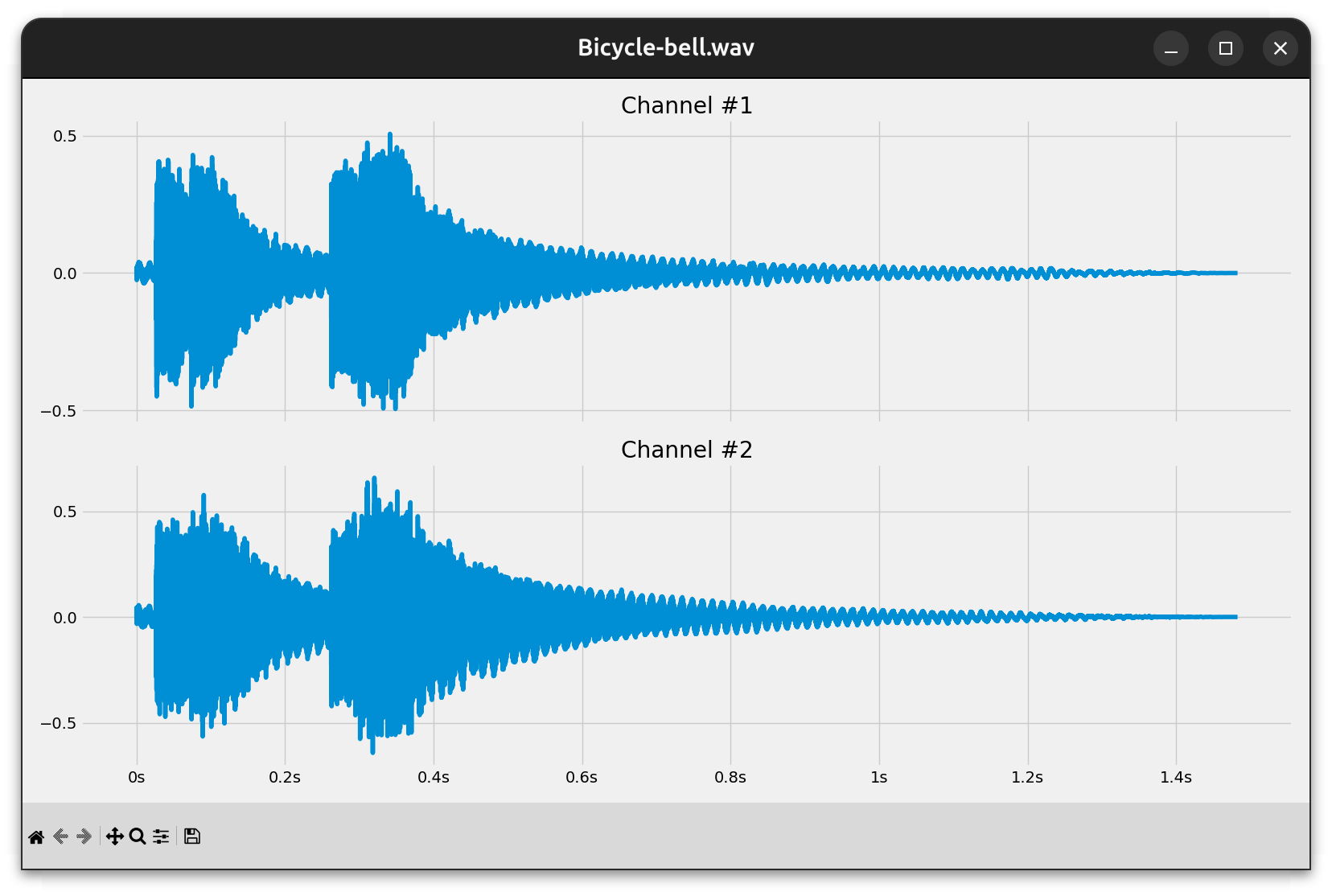
It’s a static depiction of the entire waveform, which lets you study the audio signal’s amplitude variations over time.
If you haven’t already, install Matplotlib into your virtual environment and create a Python script named plot_waveform.py outside of the waveio package. Next, paste the following source code into your new script:
plot_waveform.py
 1from argparse import ArgumentParser
 2from pathlib import Path
 3
 4import matplotlib.pyplot as plt
 5
 6from waveio import WAVReader
 7
 8def main():
 9    args = parse_args()
10    with WAVReader(args.path) as wav:
11        plot(args.path.name, wav.metadata, wav.channels)
12
13def parse_args():
14    parser = ArgumentParser(description="Plot the waveform of a WAV file")
15    parser.add_argument("path", type=Path, help="path to the WAV file")
16    return parser.parse_args()
17
18def plot(filename, metadata, channels):
19    fig, ax = plt.subplots(
20        nrows=metadata.num_channels,
21        ncols=1,
22        figsize=(16, 9),
23        sharex=True,
24    )
25
26    if isinstance(ax, plt.Axes):
27        ax = [ax]
28
29    for i, channel in enumerate(channels):
30        ax[i].set_title(f"Channel #{i + 1}")
31        ax[i].set_yticks([-1, -0.5, 0, 0.5, 1])
32        ax[i].plot(channel)
33
34    fig.canvas.manager.set_window_title(filename)
35    plt.tight_layout()
36    plt.show()
37
38if __name__ == "__main__":
39    main()
You use the argparse module to read your script’s arguments from the command line. Currently, the script expects only one positional argument, which is the path pointing to a WAV file somewhere on your disk. You use the pathlib.Path data type to represent that file path.
Following the name-main idiom, you call your main() function, which is the script’s entry point, at the bottom of the file. After parsing the command-line arguments and opening the corresponding WAV file with your WAVReader object, you can proceed and plot its audio content.
The plot() function performs these steps:
- Lines 19 to 24 create a figure with subplots corresponding to each channel in the WAV file. The number of channels determines the number of rows, while there’s only a single column in the figure. Each subplot shares the horizontal axis to align the waveforms when zooming or panning.
- Lines 26 and 27 ensure that the
axvariable is a sequence ofAxesby wrapping that variable in a list when there’s only one channel in the WAV file. - Lines 29 to 32 loop through the audio channels, setting the title of each subplot to the corresponding channel number and using fixed y-ticks for consistent scaling. Finally, they plot the waveform for the current channel on its respective
Axesobject. - Lines 34 to 36 set the window title, make the subplots fit nicely in the figure, and then display the plot on the screen.
To show the number of seconds on the horizontal axis shared by the subplots, you need to make a few tweaks:
plot_waveform.py
 1from argparse import ArgumentParser
 2from pathlib import Path
 3
 4import matplotlib.pyplot as plt
 5import numpy as np
 6from matplotlib.ticker import FuncFormatter
 7
 8from waveio import WAVReader
 9
10# ...
11
12def plot(filename, metadata, channels):
13    fig, ax = plt.subplots(
14        nrows=metadata.num_channels,
15        ncols=1,
16        figsize=(16, 9),
17        sharex=True,
18    )
19
20    if isinstance(ax, plt.Axes):
21        ax = [ax]
22
23    time_formatter = FuncFormatter(format_time)
24    timeline = np.linspace(
25        start=0,
26        stop=metadata.num_seconds,
27        num=metadata.num_frames
28    )
29
30    for i, channel in enumerate(channels):
31        ax[i].set_title(f"Channel #{i + 1}")
32        ax[i].set_yticks([-1, -0.5, 0, 0.5, 1])
33        ax[i].xaxis.set_major_formatter(time_formatter)
34        ax[i].plot(timeline, channel)
35
36    fig.canvas.manager.set_window_title(filename)
37    plt.tight_layout()
38    plt.show()
39
40def format_time(instant, _):
41    if instant < 60:
42        return f"{instant:g}s"
43    minutes, seconds = divmod(instant, 60)
44    return f"{minutes:g}m {seconds:02g}s"
45
46if __name__ == "__main__":
47    main()
By calling NumPy’s linspace() on lines 24 to 28, you calculate the timeline comprising evenly distributed time instants measured in seconds. The number of these time instants equals the number of audio frames, letting you plot them together on line 34. As a result, the number of seconds on the horizontal axis matches the respective amplitude values.
Additionally, you define a custom formatter function for your timeline and hook it up to the shared horizontal axis. Your function implemented on lines 40 to 44 makes the tick labels show the time unit when needed. To only show significant digits, you use the letter g as the format specifier in the f-strings.
As the icing on the cake, you can apply one of the available styles that come with Matplotlib to make the resulting plot look more appealing:
plot_waveform.py
# ...

def plot(filename, metadata, channels):
    try:
        plt.style.use("fivethirtyeight")
    except OSError:
        pass  # Fall back to the default style

    fig, ax = plt.subplots(
        nrows=metadata.num_channels,
        ncols=1,
        figsize=(16, 9),
        sharex=True,
    )

    # ...

# ...
In this case, you pick a style sheet inspired by the visualizations found on the FiveThirtyEight website, which specializes in opinion poll analysis. If this style is unavailable, then you can fall back on Matplotlib’s default style.
Go ahead and test your plotting script against mono, stereo, and potentially even surround sound files of varying lengths.
Once you open a larger WAV file, the amount of information will make it difficult to examine fine details. While the Matplotlib user interface provides zooming and panning tools, it can be quicker to slice audio frames to the time range of interest before plotting. Later, you’ll use this technique to animate your visualizations!
Read a Slice of Audio Frames
If you have a particularly long audio file, then you can reduce the time it takes to load and decode the underlying data by skipping and narrowing down the range of audio frames of interest:
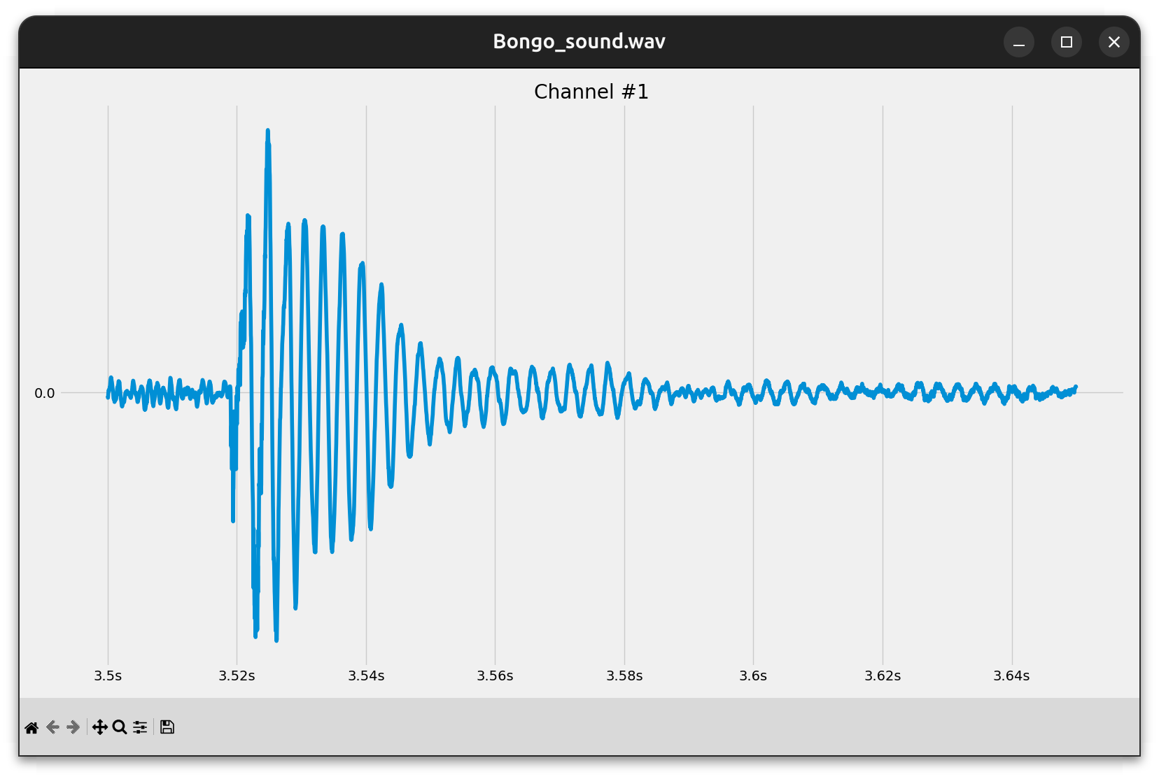
This waveform starts at three and a half seconds, and lasts about a hundred and fifty milliseconds. Now you’re about to implement this slicing feature.
Modify your plotting script to accept two optional arguments, marking the start and end of a timeline slice. Both should be expressed in seconds, which you’ll later translate to audio frame indices in the WAV file:
plot_waveform.py
# ...

def parse_args():
    parser = ArgumentParser(description="Plot the waveform of a WAV file")
    parser.add_argument("path", type=Path, help="path to the WAV file")
    parser.add_argument(
        "-s",
        "--start",
        type=float,
        default=0.0,
        help="start time in seconds (default: 0.0)",
    )
    parser.add_argument(
        "-e",
        "--end",
        type=float,
        default=None,
        help="end time in seconds (default: end of file)",
    )
    return parser.parse_args()

# ...
When you don’t specify the start time with -s or --start, then your script assumes you want to begin reading audio frames from the very beginning at zero seconds. On the other hand, the default value for the -e or --end argument is equal to None, which you’ll treat as the total duration of the entire file.
Note: You can supply negative values for either or both arguments to indicate offsets from the end of the WAV file. For example, --start -0.5 would reveal the last half a second of the waveform.
Next, you’ll want to plot the waveforms of all audio channels sliced to the specified time range. You’ll implement the slicing logic inside a new method in your WAVReader class, which you can call now:
plot_waveform.py
# ...

def main():
    args = parse_args()
    with WAVReader(args.path) as wav:
        plot(
            args.path.name,
            wav.metadata,
            wav.channels_sliced(args.start, args.end)
        )

# ...
You’ve essentially replaced a reference to the .channels property with a call to the .channels_sliced() method and passed your new command-line arguments—or their default values—to it. When you omit the --start and --end parameters, your script should work as before, plotting the entire waveform.
As you plot a slice of audio frames within your channels, you’ll also want to match the timeline with the size of that slice. In particular, your timeline may no longer start at zero seconds, and it may end earlier than the full duration of the file. To adjust for that, you can attach a range() of frame indices to your channels and use it to calculate the new timeline:
plot_waveform.py
# ...

def plot(filename, metadata, channels):
    # ...

    time_formatter = FuncFormatter(format_time)
    timeline = np.linspace(
        channels.frames_range.start / metadata.frames_per_second,
        channels.frames_range.stop / metadata.frames_per_second,
        len(channels.frames_range)
    )

    # ...

# ...
Here, you convert integer indices of audio frames to their corresponding time instants in seconds from the beginning of the file. At this point, you’re done with editing the plotting script. It’s time to update your waveio.reader module now.
To allow for reading the WAV file from an arbitrary frame index, you can take advantage of the wave.Wave_read object’s .setpos() method instead of rewinding to the file’s beginning. Go ahead and replace .rewind() with .setpos(), add a new parameter, start_frame, to your internal ._read() method, and give it a default value of None:
waveio/reader.py
# ...

class WAVReader:
    # ...

    @cached_property
    @reshape("rows")
    def frames(self):
        return self._read(self.metadata.num_frames, start_frame=0)

    # ...

    def _read(self, max_frames=None, start_frame=None):
        if start_frame is not None:
            self._wav_file.setpos(start_frame)
        frames = self._wav_file.readframes(max_frames)
        return self.metadata.encoding.decode(frames)
When you call ._read() with some value for this new parameter, you’ll move the internal pointer to that position. Otherwise, you’ll commence from the last known position, which means that the function won’t rewind the pointer for you anymore. Therefore, you must explicitly pass zero as the starting frame when you read all frames eagerly in the corresponding property.
Now, define the .channels_sliced() method that you called before in your plotting script:
waveio/reader.py
# ...

class WAVReader:
    # ...

    @reshape("columns")
    def channels_sliced(self, start_seconds=0.0, end_seconds=None):
        if end_seconds is None:
            end_seconds = self.metadata.num_seconds
        frames_slice = slice(
            round(self.metadata.frames_per_second * start_seconds),
            round(self.metadata.frames_per_second * end_seconds)
        )
        frames_range = range(*frames_slice.indices(self.metadata.num_frames))
        values = self._read(len(frames_range), frames_range.start)
        return ArraySlice(values, frames_range)

    # ...

# ...
This method accepts two optional parameters, which represent the start and end of the WAV file in seconds. When you don’t specify the end one, it defaults to the total duration of the file.
Inside that method, you create a slice() object of the corresponding frame indices. To account for negative values, you expand the slice into a range() object by providing the total number of frames. Then, you use that range to read and decode a slice of audio frames into amplitude values.
Before returning from the function, you combine the sliced amplitudes and the corresponding range of frame indices in a custom wrapper for the NumPy array. This wrapper will behave just like a regular array, but it’ll also expose the .frames_range attribute that you can use to calculate the correct timeline for plotting.
This is the wrapper’s implementation that you can add to the reader module before your WAVReader class definition:
waveio/reader.py
# ...

class ArraySlice:
    def __init__(self, values, frames_range):
        self.values = values
        self.frames_range = frames_range

    def __iter__(self):
        return iter(self.values)

    def __getattr__(self, name):
        return getattr(self.values, name)

    def reshape(self, *args, **kwargs):
        reshaped = self.values.reshape(*args, **kwargs)
        return ArraySlice(reshaped, self.frames_range)

    @property
    def T(self):
        return ArraySlice(self.values.T, self.frames_range)

# ...
Whenever you try to access one of NumPy array’s attributes on your wrapper, the .__getattr__() method delegates to the .values field, which is the original array of amplitude levels. The .__iter__() method makes it possible to loop over your wrapper.
Unfortunately, you also need to override the array’s .reshape() method and the .T property, which you use in your @reshape decorator. That’s because they return plain NumPy arrays instead of your wrapper, effectively erasing the extra information about the range of frame indices. You can address this problem by wrapping their results again.
Now, you can zoom in on a particular slice of audio frames in all channels by supplying the --start and --end parameters:
$ python plot_waveform.py Bongo_sound.wav --start 3.5 --end 3.65
The above command plots the waveform that you saw in the screenshot at the beginning of this section.
Since you know how to load a fraction of audio frames at a time, you can read huge WAV files or even online audio streams incrementally. This enables animating a live preview of the sound in the time and frequency domains, which you’ll do next.
Process Large WAV Files in Python Efficiently
Because WAV files typically contain uncompressed data, it’s not uncommon for them to reach considerable sizes. This can make their processing extremely slow or even prevent you from fitting the entire file into memory at once.
In this part of the tutorial, you’ll read a relatively big WAV file in chunks using lazy evaluation to improve memory use efficiency. Additionally, you’ll write a continuous stream of audio frames sourced from an Internet radio station to a local WAV file.
For testing purposes, you can grab a large enough WAV file from an artist who goes by the name Waesto on various social media platforms:
Hi! I’m Waesto, a music producer creating melodic music for content creators to use here on YouTube or other social media. You may use the music for free as long as I am credited in the description! (Source)
To download Waesto’s music in the WAV file format, you need to subscribe to the artist’s YouTube channel or follow them on other social media. Their music is generally copyrighted but free to use as long as it’s credited appropriately.
You’ll find a direct download link and the credits in each video description on YouTube. For example, one of the artist’s early songs, entitled Sleepless, provides a link to the corresponding WAV file hosted on the Hypeddit platform. It’s a 24-bit uncompressed PCM stereo audio sampled at 44.1 kHz, which weighs in at about forty-six megabytes.
Feel free to use any of Waesto’s tracks or a completely different WAV file that appeals to you. Just remember that it must be a large one.
Animate the Waveform Graph in Real Time
Instead of plotting a static waveform of the whole or a part of a WAV file, you can use the sliding window technique to visualize a small segment of the audio as it plays. This will create an interesting oscilloscope effect by updating the plot in real-time:
Such a dynamic representation of sound is an example of music visualization akin to the visual effects you’d find in the classic Winamp player.
You don’t need to modify your WAVReader object, which already provides the means necessary to jump to a given position in a WAV file. As earlier, you’ll create a new script file to handle the visualization. Name the script plot_oscilloscope.py and fill it with the source code below:
plot_oscilloscope.py
from argparse import ArgumentParser
from pathlib import Path

from waveio import WAVReader

def main():
    args = parse_args()
    with WAVReader(args.path) as wav:
        animate(
            args.path.name,
            args.seconds,
            slide_window(args.seconds, wav),
        )

def parse_args():
    parser = ArgumentParser(description="Animate WAV file waveform")
    parser.add_argument("path", type=Path, help="path to the WAV file")
    parser.add_argument(
        "-s",
        "--seconds",
        type=float,
        default=0.05,
        help="sliding window size in seconds",
    )
    return parser.parse_args()

def slide_window(window_seconds, wav):
    ...

def animate(filename, seconds, windows):
    ...

if __name__ == "__main__":
    try:
        main()
    except KeyboardInterrupt:
        print("Aborted")
The overall structure of the script remains analogous to the one you created in the previous section. You start by parsing the command-line arguments including the path to a WAV file and an optional sliding window’s duration, which defaults to fifty milliseconds. The shorter the window, the fewer amplitudes will show up on the screen. At the same time, the animation will become smoother by refreshing each frame more often.
Note: There are two placeholder functions, animate() and slide_window(), which you’ll implement soon.
After opening the specified WAV file for reading, you call animate() with the filename, the window’s duration, and a lazily-evaluated sequence of windows obtained from slide_window(), which is a generator function:
plot_oscilloscope.py
from argparse import ArgumentParser
from pathlib import Path

import numpy as np

from waveio import WAVReader

# ...

def slide_window(window_seconds, wav):
    num_windows = round(wav.metadata.num_seconds / window_seconds)
    for i in range(num_windows):
        begin_seconds = i * window_seconds
        end_seconds = begin_seconds + window_seconds
        channels = wav.channels_sliced(begin_seconds, end_seconds)
        yield np.mean(tuple(channels), axis=0)

# ...
A single window is nothing more than a slice of audio frames that you learned to read earlier. Given the total number of seconds in the file and the window’s duration, this function calculates the window count and iterates over a range of indices. For each window, it determines where it begins and ends on the timeline to slice the audio frames appropriately. Finally, it yields the average amplitude from all channels at the given time instant.
The animation part consumes your generator of windows and plots each of them with a slight delay:
plot_oscilloscope.py
from argparse import ArgumentParser
from pathlib import Path

import matplotlib.pyplot as plt
import numpy as np

from waveio import WAVReader

# ...

def animate(filename, seconds, windows):
    try:
        plt.style.use("dark_background")
    except OSError:
        pass  # Fall back to the default style

    fig, ax = plt.subplots(figsize=(16, 9))
    fig.canvas.manager.set_window_title(filename)

    plt.tight_layout()
    plt.box(False)

    for window in windows:
        plt.cla()
        ax.set_xticks([])
        ax.set_yticks([])
        ax.set_ylim(-1.0, 1.0)
        plt.plot(window)
        plt.pause(seconds)

# ...
First, you pick Matplotlib’s theme with a dark background for a more dramatic visual effect. Then, you set up the figure and an Axes object, remove the default border around your visualization, and iterate over the windows. On each iteration, you clear the plot, hide the ticks, and fix the vertical scale to keep it consistent across all windows. After plotting the current window, you pause the loop for the duration of a single window.
Here’s how you can start the animation from the command line to visualize the downloaded WAV file with your favorite music:
$ python plot_oscilloscope.py /path/to/some_music.wav
The oscilloscope effect can give you insight into the temporal dynamics of an audio file in the time domain. Next up, you’ll reuse most of this code to show spectral changes in the frequency domain of each window.
Show a Real-Time Spectrogram Visualization
While a waveform tells you about the amplitude changes over time, a spectrogram can provide a visual representation of how the intensities of different frequency bands vary with time. Media players often include a real-time visualization of the music, which looks similar to the one below:
The width of each vertical bar corresponds to a range of frequencies or a frequency band, with its height depicting the relative energy level within that band at any given moment. Frequencies increase from left to right, with lower frequencies represented on the left side of the spectrum and higher frequencies toward the right.
Note: To achieve such an engaging effect in Python, you’ll need to calculate the short-term Fourier transform, which is a sequence of Discrete Fourier Transforms (DFT) computed separately for each audio segment enclosed by the sliding window. You’ll use NumPy to leverage the Fast Fourier Transform (FFT) algorithm for improved performance.
That said, calculating FFT remains a computationally demanding task. So, if your animation ends up looking choppy, then try to reduce the number of frequency bands by decreasing the sliding window’s size.
Now copy the entire source code from plot_oscilloscope.py and paste it into a new script named plot_spectrogram.py, which you’ll modify to create a new visualization of the WAV file.
Because you’ll be calculating the FFT of short audio segments, you’ll want to overlap adjacent segments to minimize the spectral leakage caused by abrupt discontinuities at the edges. They introduce phantom frequencies into the spectrum, which don’t exist in the actual signal. An overlay of fifty percent is a good starting point, but you can make it configurable through another command-line argument:
plot_spectrogram.py
# ...

def parse_args():
    parser = ArgumentParser(description="Animate WAV file spectrogram")
    parser.add_argument("path", type=Path, help="path to the WAV file")
    parser.add_argument(
        "-s",
        "--seconds",
        type=float,
        default=0.0015,
        help="sliding window size in seconds",
    )
    parser.add_argument(
        "-o",
        "--overlap",
        choices=range(100),
        default=50,
        type=int,
        help="sliding window overlap as a percentage",
    )
    return parser.parse_args()

# ...
The --overlap argument’s value must be an integer number between zero inclusive and one hundred exclusive, representing a percentage. The greater the overlap, the smoother the animation will appear.
Note: Unlike the waveform, a spectrum visualization is much more resource-intensive to compute, so you’ll have to reduce the window duration to as little as a few milliseconds! That’s why you’ve adjusted the default value for the --seconds argument.
You can now modify your slide_window() function to accept that overlap percentage as an additional parameter:
plot_spectrogram.py
# ...

def slide_window(window_seconds, overlap_percentage, wav):
    step_seconds = window_seconds * (1 - overlap_percentage / 100)
    num_windows = round(wav.metadata.num_seconds / step_seconds)
    for i in range(num_windows):
        begin_seconds = i * step_seconds
        end_seconds = begin_seconds + window_seconds
        channels = wav.channels_sliced(begin_seconds, end_seconds)
        yield np.mean(tuple(channels), axis=0)

# ...
Instead of moving the window by its whole duration as before, you introduce a step that can be smaller, resulting in a greater number of windows in total. On the other hand, when the overlap percentage is zero, you arrange the windows next to each other without any overlap between them.
You can now pass the overlap requested at the command line to your generator function, as well as the animate() function:
plot_spectrogram.py
# ...

def main():
    args = parse_args()
    with WAVReader(args.path) as wav:
        animate(
            args.path.name,
            args.seconds,
            args.overlap,
            fft(slide_window(args.seconds, args.overlap, wav), wav),
        )

# ...
You’ll need to know the overlap to adjust the animation’s speed accordingly. Notice that you wrap the call to slide_window() with another call to a new function, fft(), which calculates the frequencies and their corresponding magnitudes in the sliding window:
plot_spectrogram.py
 1# ...
 2
 3def fft(windows, wav):
 4    sampling_period = 1 / wav.metadata.frames_per_second
 5    for window in windows:
 6        frequencies = np.fft.rfftfreq(window.size, sampling_period)
 7        magnitudes = np.abs(
 8            np.fft.rfft(
 9                (window - np.mean(window)) * np.blackman(window.size)
10            )
11        )
12        yield frequencies, magnitudes
13
14# ...
There’s a lot going on, so it’ll help to break this function down line by line:
- Line 4 calculates the sampling period, which is the time interval between audio samples in the file, as the reciprocal of the frame rate.
- Line 6 uses your window size and the sampling period to determine the frequencies in the audio. Note that the highest frequency in the spectrum will be exactly half the frame rate due to the Nyquist–Shannon theorem mentioned earlier.
- Lines 7 to 11 find the magnitudes of each frequency determined on line 6. Before performing the Fourier transform of the wave amplitudes, you subtract the mean value, often referred to as the DC bias, which is the non-varying part of the signal representing the zero-frequency term in the Fourier transform. Additionally, you apply a window function to smooth out the window’s edges even more.
- Line 12 yields a tuple comprising the frequencies and their corresponding magnitudes.
Lastly, you must update your animation code to draw a bar plot of frequencies at each sliding window position:
plot_spectrogram.py
def animate(filename, seconds, overlap_percentage, windows):
    try:
        plt.style.use("dark_background")
    except OSError:
        pass  # Fall back to the default style

    fig, ax = plt.subplots(figsize=(16, 9))
    fig.canvas.manager.set_window_title(filename)

    plt.tight_layout()
    plt.box(False)

    bar_gap = 0.25
    for frequencies, magnitudes in windows:
        bar_width = (frequencies[-1] / frequencies.size) * (1 - bar_gap)
        plt.cla()
        ax.set_xticks([])
        ax.set_yticks([])
        ax.set_xlim(-bar_width / 2, frequencies[-1] - bar_width / 2)
        ax.set_ylim(0, np.max(magnitudes))
        ax.bar(frequencies, magnitudes, width=bar_width)
        plt.pause(seconds * (1 - overlap_percentage / 100))
You pass the overlap percentage in order to adjust the animation’s delay between subsequent frames. Then, you iterate over the frequencies and their magnitudes, plotting them as vertical bars spaced out by the desired gap. You also update the axis limits accordingly.
Run the command below to kick off the spectrogram’s animation:
$ python plot_spectrogram.py file.wav --seconds 0.001 --overlap 95
Play around with the sliding window’s duration and the overlap percentage to see how they affect your animation. Once you get bored and are thirsty for more practical uses of the wave module in Python, you can step up your game by trying something more challenging!
Record an Internet Radio Station as a WAV File
Up until now, you’ve been using abstractions from your waveio package to read and decode WAV files conveniently, which allowed you to focus on higher-level tasks. It’s now time to add the missing piece of the puzzle and implement the WAVReader type’s counterpart. You’ll make a lazy writer object capable of writing chunks of audio data into a WAV file.
For this task, you’ll undertake a hands-on example—stream ripping an Internet radio station to a local WAV file.
Note: Always check the terms of service to see if it’s legal to record a particular live stream, especially with copyrighted content.
If you have a premium account on di.fm, then you can use your unique security token to connect to the broadcaster’s server using third-party software. That includes your custom Python script. Alternatively, you might be able to find a public radio station that permits recording of their broadcast for personal and non-commercial use. For example, check out the list of NPR stations.
To simplify connecting to an online stream, you’ll use a tiny helper class to obtain audio frames in real time. Expand the collapsible section below to reveal the source code and instructions on using the RadioStream class that you’ll need later:
The following code depends on pyav, which is a Python binding for the FFmpeg library. After installing both libraries, put this module next to your stream-ripping script so that you can import the RadioStream class from it:
stream.py
import av

from waveio.encoding import PCMEncoding
from waveio.metadata import WAVMetadata

class RadioStream:
    def __init__(self, stream_url):
        self.container = av.open(stream_url)
        self.metadata = get_metadata(self.container)

    def __enter__(self):
        return self

    def __exit__(self, *args, **kwargs):
        self.container.close()

    def __iter__(self):
        for chunk in self.container.decode():
            yield chunk.to_ndarray()

def get_metadata(container):
    (audio_stream,) = container.streams.audio
    num_channels = audio_stream.channels
    bytes_per_sample = audio_stream.format.bytes // num_channels
    return WAVMetadata(
        encoding=PCMEncoding(bytes_per_sample),
        frames_per_second=audio_stream.rate,
        num_channels=num_channels,
    )
The module defines the RadioStream class, which takes the URL address of an Internet radio station. It exposes the underlying WAV metadata and lets you iterate over the audio channels in chunks. Each chunk is represented as a familiar NumPy array.
Now, create the writer module in your waveio package and use the code below to implement the functionality for incrementally writing audio frames into a new WAV file:
waveio/writer.py
import wave

class WAVWriter:
    def __init__(self, metadata, path):
        self.metadata = metadata
        self._wav_file = wave.open(str(path), mode="wb")
        self._wav_file.setframerate(metadata.frames_per_second)
        self._wav_file.setnchannels(metadata.num_channels)
        self._wav_file.setsampwidth(metadata.encoding)

    def __enter__(self):
        return self

    def __exit__(self, *args, **kwargs):
        self._wav_file.close()

    def append_channels(self, channels):
        self.append_amplitudes(channels.T.reshape(-1))

    def append_amplitudes(self, amplitudes):
        frames = self.metadata.encoding.encode(amplitudes)
        self._wav_file.writeframes(frames)
The WAVWriter class takes a WAVMetadata instance and a path to the output WAV file. It then opens the file for writing in binary mode and uses the metadata to set the appropriate header values. Note that the number of audio frames remains unknown at this stage so instead of specifying it, you let the wave module update it later when the file’s closed.
Just like the reader, your writer object follows the context manager protocol. When you enter a new context using the with keyword, the new WAVWriter instance will return itself. Conversely, exiting the context will ensure that the WAV file gets properly closed even if an error occurs.
After creating an instance of WAVWriter, you can add a chunk of data to your WAV file by calling .append_channels() with a two-dimensional NumPy array of channels as an argument. The method will reshape the channels into a flat array of amplitude values and encode them using the format specified in the metadata.
Remember to add the following import statement to your waveio package’s __init__.py file before moving on:
waveio/__init__.py
from waveio.reader import WAVReader
from waveio.writer import WAVWriter

__all__ = ["WAVReader", "WAVWriter"]
This enables direct importing of the WAVWriter class from your package, bypassing the intermediate writer module.
Finally, you can connect the dots and build your very own stream ripper in Python:
record_stream.py
from argparse import ArgumentParser

from stream import RadioStream
from waveio import WAVWriter

def main():
    args = parse_args()
    with RadioStream(args.stream_url) as radio_stream:
        with WAVWriter(radio_stream.metadata, args.output) as writer:
            for channels_chunk in radio_stream:
                writer.append_channels(channels_chunk)

def parse_args():
    parser = ArgumentParser(description="Record an Internet radio stream")
    parser.add_argument("stream_url", help="URL address of the stream")
    parser.add_argument(
        "-o",
        "--output",
        metavar="path",
        required=True,
        type=str,
        help="path to the output WAV file",
    )
    return parser.parse_args()

if __name__ == "__main__":
    try:
        main()
    except KeyboardInterrupt:
        print("Aborted")
You open a radio stream using the URL provided as a command-line argument and use the obtained metadata for your output WAV file. Usually, the first chunk of the stream contains information such as the media container format, encoding, frame rate, number of channels, and bit depth. Next, you loop over the stream and append each decoded chunk of audio channels to the file, capturing the volatile moment of a live broadcast.
Here’s an example command showing how you can record the Classic EuroDance channel:
$ RADIO_URL=http://prem2.di.fm:80/classiceurodance?your-secret-token
$ python record_stream.py "$RADIO_URL" --output ripped.wav
Note that you won’t see any output while the program’s running. To stop recording the chosen radio station and exit your script, hit Ctrl+C on Linux and Windows or Cmd+C if you’re on macOS.
While you can write a WAV file in chunks now, you haven’t actually implemented proper logic for the analogous lazy reading before. Even though you can load a slice of audio data delimited by the given timestamps, it isn’t the same as iterating over a sequence of fixed-size chunks in a loop. You’ll have the opportunity to implement such a chunk-based reading mechanism in what comes next.
Widen the Stereo Field of a WAV File
In this section, you’ll simultaneously read a chunk of audio frames from one WAV file and write its modified version to another file in a lazy fashion. To do that, you’re going to need to enhance your WAVReader object by adding the following method:
waveio/reader.py
# ...

class WAVReader:
    DEFAULT_MAX_FRAMES = 1024

    # ...

    @reshape("columns")
    def channels_lazy(self, max_frames=DEFAULT_MAX_FRAMES):
        self._wav_file.rewind()
        while True:
            chunk = self._read(max_frames)
            if chunk.size == 0:
                break
            yield chunk

# ...
It’s a generator method, which takes an optional parameter indicating the maximum number of audio frames to read at a time. This parameter falls back to a default value defined in a constant class attribute. After rewinding the file to its starting position, the method enters an infinite loop, which reads and yields the subsequent chunks of channel data until there are no more audio frames to read.
Note: If a chunk was a regular Python list or another sequence type, then you could simplify your function by using the Walrus operator (:=). More specifically, you could directly evaluate the chunk as the loop’s continuation condition:
while chunk := self._read(max_frames):
This relies on the implicit conversion of an expression to a Boolean value in a logical context. Python generally treats empty collections as falsy while non-empty ones as truthy. However, that’s not the case for NumPy arrays, which deem such behavior ambiguous and forbid it altogether.
Like most other methods and properties in this class, .channels_lazy() is decorated with @reshape to arrange the decoded amplitudes in a more convenient way. Unfortunately, this decorator acts on a NumPy array, whereas your new method returns a generator object. To make them compatible, you must update the decorator’s definition by handling two cases:
waveio/reader.py
import inspect
import wave
from functools import cached_property, wraps

from waveio.encoding import PCMEncoding
from waveio.metadata import WAVMetadata

def reshape(shape):
    if shape not in ("rows", "columns"):
        raise ValueError("shape must be either 'rows' or 'columns'")

    def decorator(method):
        if inspect.isgeneratorfunction(method):
            @wraps(method)
            def wrapper(self, *args, **kwargs):
                for values in method(self, *args, **kwargs):
                    reshaped = values.reshape(-1, self.metadata.num_channels)
                    yield reshaped if shape == "rows" else reshaped.T
        else:
            @wraps(method)
            def wrapper(self, *args, **kwargs):
                values = method(self, *args, **kwargs)
                reshaped = values.reshape(-1, self.metadata.num_channels)
                return reshaped if shape == "rows" else reshaped.T
        return wrapper

    return decorator

# ...
You use the inspect module to determine if your decorator wraps a regular method or a generator method. Both wrappers do the same thing, but the generator wrapper yields the reshaped values in each iteration, while the regular method wrapper returns them.
Lastly, you can add another property that’ll tell you whether your WAV file is a stereo one or not:
waveio/reader.py
# ...

class WAVReader:
    # ...

    @cached_property
    def stereo(self):
        return 2 == self.metadata.num_channels

    # ...

# ...
It checks if the number of channels declared in the file’s header is equal to two.
With these changes in place, you can read your WAV files in chunks and start applying various sound effects. For example, you can widen or narrow the stereo field of an audio file to enhance or diminish the sensation of space. One such technique involves converting a conventional stereo signal comprising the left and right channels into the mid and side channels.
The mid channel (M) contains a monophonic component that’s common to both sides, while the side channel (S) captures the differences between the left (L) and right (R) channels. You can convert between both representations using the following formulas:

When you’ve separated the side channel, you can boost it independently from the mid one before recombining them to the left and right channels again. To see this in action, create a script named stereo_booster.py that takes paths to the input and output WAV files as arguments with an optional strength parameter:
stereo_booster.py
from argparse import ArgumentParser

def main():
    args = parse_args()

def parse_args():
    parser = ArgumentParser(description="Widen the stereo field")
    parser.add_argument(
        "-i",
        "--input",
        dest="input_path",
        required=True,
        type=str,
        help="path to the input WAV file",
    )
    parser.add_argument(
        "-o",
        "--output",
        dest="output_path",
        required=True,
        type=str,
        help="path to the output WAV file",
    )
    parser.add_argument(
        "-s",
        "--strength",
        type=float,
        default=1.0,
        help="strength (defaults to 1)",
    )
    return parser.parse_args()

if __name__ == "__main__":
    try:
        main()
    except KeyboardInterrupt:
        print("Aborted")
The --strength parameter is a multiplier for the side channel. Use a value greater than one to widen the stereo field and a value between zero and one to narrow it.
Next, implement the channel conversion formulas as Python functions:
stereo_booster.py
from argparse import ArgumentParser

def main():
    args = parse_args()

def convert_to_ms(left, right):
    return (left + right) / 2, (left - right) / 2

def convert_to_lr(mid, side):
    return mid + side, mid - side

# ...
Both take two parameters corresponding to either the left and right, or the mid and side channels while returning a tuple of the converted channels.
Finally, you can open a stereo WAV file for reading, loop through its channels in chunks, and apply the explained mid-side processing:
stereo_booster.py
from argparse import ArgumentParser

from waveio import WAVReader, WAVWriter

def main():
    args = parse_args()
    with (
        WAVReader(args.input_path) as source,
        WAVWriter(source.metadata, args.output_path) as target,
    ):
        if source.stereo:
            for channels_chunk in source.channels_lazy():
                mid, side = convert_to_ms(*channels_chunk)
                left, right = convert_to_lr(mid, side * args.strength)
                target.append_channels(left, right)
        else:
            print("Only stereo WAV files are supported")

# ...
The output WAV file has the same encoding format as the input file. After converting each chunk into the mid and side channels, you convert them back to the left and right channels while boosting the side one only.
Notice that you append the modified channels as separate arguments now, whereas your radio recording script passed a single NumPy array of combined channels. To make the .append_channels() method work with both types of invocations, you can update your WAVWriter class as follows:
waveio/writer.py
import wave

import numpy as np

class WAVWriter:
    # ...

    def append_channels(self, *channels):
        match channels:
            case [combined] if combined.ndim > 1:
                self.append_amplitudes(combined.T.reshape(-1))
            case _:
                self.append_amplitudes(np.dstack(channels).reshape(-1))

    def append_amplitudes(self, amplitudes):
        frames = self.metadata.encoding.encode(amplitudes)
        self._wav_file.writeframes(frames)

    # ...

# ...
You use structural pattern matching again to differentiate between a single multi-channel array and multiple single-channel arrays, reshaping them into a flat sequence of amplitudes for encoding accordingly.
Try boosting one of the sample WAV files, such as the bicycle bell sound, by a factor of five:
$ python stereo_booster.py -i Bicycle-bell.wav -o boosted.wav -s 5
Remember to choose a stereo sound, and for the best listening experience, use your external loudspeakers instead of headphones to play back the output file. Can you hear the difference?
Conclusion
You’ve covered a lot of ground in this tutorial. After learning about the WAV file’s structure, you got to grips with Python’s wave module for reading and writing raw binary data. Then, you built your own abstractions on top of the wave module so you could think about the audio data in higher-level terms. This, in turn, allowed you to implement several practical and fun audio analysis and processing tools.
In this tutorial, you’ve learned how to:
- Read and write WAV files using pure Python
- Handle the 24-bit PCM encoding of audio samples
- Interpret and plot the underlying amplitude levels
- Record online audio streams like Internet radio stations
- Animate visualizations in the time and frequency domains
- Synthesize sounds and apply special effects
Now that you have so much experience working with WAV files in Python under your belt, you can tackle even more ambitious projects. For instance, based on your knowledge of calculating the Fourier transform and processing WAV files lazily, you can implement a vocoder effect, popularized by the German band Kraftwerk in the seventies. It’ll make your voice sound like a musical instrument or a robot!
Get Your Code: Click here to download the free sample code that shows you how to read and write WAV files in Python.
Take the Quiz: Test your knowledge with our interactive “Reading and Writing WAV Files in Python” quiz. You’ll receive a score upon completion to help you track your learning progress:
Interactive Quiz
Reading and Writing WAV Files in PythonIn this quiz, you can test your knowledge of handling WAV audio files in Python with the wave module. By applying what you've learned, you'll demonstrate your ability to synthesize sounds, analyze and visualize waveforms, create dynamic spectrograms, and enhance audio with special effects.