
Binary search is a classic algorithm in computer science. It often comes up in programming contests and technical interviews. Implementing binary search turns out to be a challenging task, even when you understand the concept. Unless you’re curious or have a specific assignment, you should always leverage existing libraries to do a binary search in Python or any other language.
In this tutorial, you’ll learn how to:
- Use the
bisectmodule to do a binary search in Python - Implement a binary search in Python both recursively and iteratively
- Recognize and fix defects in a binary search Python implementation
- Analyze the time-space complexity of the binary search algorithm
- Search even faster than binary search
This tutorial assumes you’re a student or an intermediate programmer with an interest in algorithms and data structures. At the very least, you should be familiar with Python’s built-in data types, such as lists and tuples. In addition, some familiarity with recursion, classes, data classes, and lambdas will help you better understand the concepts you’ll see in this tutorial.
Below you’ll find a link to the sample code you’ll see throughout this tutorial, which requires Python 3.7 or later to run:
Get Sample Code: Click here to get the sample code you’ll use to learn about binary search in Python in this tutorial.
Benchmarking
In the next section of this tutorial, you’ll be using a subset of the Internet Movie Database (IMDb) to benchmark the performance of a few search algorithms. This dataset is free of charge for personal and non-commercial use. It’s distributed as a bunch of compressed tab-separated values (TSV) files, which get daily updates.
To make your life easier, you can use a Python script included in the sample code. It’ll automatically fetch the relevant file from IMDb, decompress it, and extract the interesting pieces:
$ python download_imdb.py
Fetching data from IMDb...
Created "names.txt" and "sorted_names.txt"
Be warned that this will download and extract approximately 600 MB of data, as well as produce two additional files, which are about half of that in size. The download, as well as the processing of this data, might take a minute or two to complete.
Download IMDb
To manually obtain the data, navigate your web browser to https://datasets.imdbws.com/ and grab the file called name.basics.tsv.gz, which contains the records of actors, directors, writers, and so on. When you decompress the file, you’ll see the following content:
nconst     primaryName      birthYear  deathYear  (...)
nm0000001  Fred Astaire     1899       1987       (...)
nm0000002  Lauren Bacall    1924       2014       (...)
nm0000003  Brigitte Bardot  1934       \N         (...)
nm0000004  John Belushi     1949       1982       (...)
It has a header with the column names in the first line, followed by data records in each of the subsequent lines. Each record contains a unique identifier, a full name, birth year, and a few other attributes. These are all delimited with a tab character.
There are millions of records, so don’t try to open the file with a regular text editor to avoid crashing your computer. Even specialized software such as spreadsheets can have problems opening it. Instead, you might take advantage of the high-performance data grid viewer included in JupyterLab, for example.
Read Tab-Separated Values
There are a few ways to parse a TSV file. For example, you can read it with Pandas, use a dedicated application, or leverage a few command-line tools. However, it’s recommended that you use the hassle-free Python script included in the sample code.
Note: As a rule of thumb, you should avoid parsing files manually because you might overlook edge cases. For example, in one of the fields, the delimiting tab character could be used literally inside quotation marks, which would break the number of columns. Whenever possible, try to find a relevant module in the standard library or a trustworthy third-party one.
Ultimately, you want to end up with two text files at your disposal:
names.txtsorted_names.txt
One will contain a list of names obtained by cutting out the second column from the original TSV file:
Fred Astaire
Lauren Bacall
Brigitte Bardot
John Belushi
Ingmar Bergman
...
The second one will be the sorted version of this.
Once both files are ready, you can load them into Python using this function:
def load_names(path):
    with open(path) as text_file:
        return text_file.read().splitlines()

names = load_names('names.txt')
sorted_names = load_names('sorted_names.txt')
This code returns a list of names pulled from the given file. Note that calling .splitlines() on the resulting string removes the trailing newline character from each line. As an alternative, you could call text_file.readlines(), but that would keep the unwanted newlines.
Measure the Execution Time
To evaluate the performance of a particular algorithm, you can measure its execution time against the IMDb dataset. This is usually done with the help of the built-in time or timeit modules, which are useful for timing a block of code.
You could also define a custom decorator to time a function if you wanted to. The sample code provided uses time.perf_counter_ns(), introduced in Python 3.7, because it offers high precision in nanoseconds.
Understanding Search Algorithms
Searching is ubiquitous and lies at the heart of computer science. You probably did several web searches today alone, but have you ever wondered what searching really means?
Search algorithms take many different forms. For example, you can:
- Do a full-text search
- Match strings with fuzzy searching
- Find the shortest path in a graph
- Query a database
- Look for a minimum or maximum value
In this tutorial, you’ll learn about searching for an element in a sorted list of items, like a phone book. When you search for such an element, you might be asking one of the following questions:
| Question | Answer |
|---|---|
| Is it there? | Yes |
| Where is it? | On the 42nd page |
| Which one is it? | A person named John Doe |
The answer to the first question tells you whether an element is present in the collection. It always holds either true or false. The second answer is the location of an element within the collection, which may be unavailable if that element was missing. Finally, the third answer is the element itself, or a lack of it.
Note: Sometimes there might be more than one correct answer due to duplicate or similar items. For example, if you have a few contacts with the same name, then they will all fit your search criteria. At other times, there might only be an approximate answer or no answer at all.
In the most common case, you’ll be searching by value, which compares elements in the collection against the exact one you provide as a reference. In other words, your search criteria are the entire element, such as a number, a string, or an object like a person. Even the tiniest difference between the two compared elements won’t result in a match.
On the other hand, you can be more granular with your search criteria by choosing some property of an element, such as a person’s last name. This is called searching by key because you pick one or more attributes to compare. Before you dive into binary search in Python, let’s take a quick look at other search algorithms to get a bigger picture and understand how they work.
Random Search
How might you look for something in your backpack? You might just dig your hand into it, pick an item at random, and see if it’s the one you wanted. If you’re out of luck, then you put the item back, rinse, and repeat. This example is a good way to understand random search, which is one of the least efficient search algorithms. The inefficiency of this approach stems from the fact that you’re running the risk of picking the same wrong thing multiple times.
Note: Funnily enough, this strategy could be the most efficient one, in theory, if you were very lucky or had a small number of elements in the collection.
The fundamental principle of this algorithm can be expressed with the following snippet of Python code:
import random

def find(elements, value):
    while True:
        random_element = random.choice(elements)
        if random_element == value:
            return random_element
The function loops until some element chosen at random matches the value given as input. However, this isn’t very useful because the function returns either None implicitly or the same value it already received in a parameter.
Note that this function never terminates for missing values. You can find the full implementation, which takes such corner cases into consideration, in the sample code available for download at the link below:
Get Sample Code: Click here to get the sample code you’ll use to learn about binary search in Python in this tutorial.
For microscopic datasets, the random search algorithm appears to be doing its job reasonably fast:
>>> from search.random import *  # Sample code to download
>>> fruits = ['orange', 'plum', 'banana', 'apple']
>>> contains(fruits, 'banana')
True
>>> find_index(fruits, 'banana')
2
>>> find(fruits, key=len, value=4)
'plum'
However, imagine having to search like that through millions of elements! Here’s a quick rundown of a performance test that was done against the IMDb dataset:
| Search Term | Element Index | Best Time | Average Time | Worst Time |
|---|---|---|---|---|
| Fred Astaire | 0 |
0.74s |
21.69s |
43.16s |
| Alicia Monica | 4,500,000 |
1.02s |
26.17s |
66.34s |
| Baoyin Liu | 9,500,000 |
0.11s |
17.41s |
51.03s |
| missing | N/A |
5m 16s |
5m 40s |
5m 54s |
Unique elements at different memory locations were specifically chosen to avoid bias. Each term was searched for ten times to account for the randomness of the algorithm and other factors such as garbage collection or system processes running in the background.
Note: If you’d like to conduct this experiment yourself, then refer back to the instructions in the introduction to this tutorial. To measure the performance of your code, you can use the built-in time and timeit modules, or you can time functions with a custom decorator.
The algorithm has a non-deterministic performance. While the average time to find an element doesn’t depend on its whereabouts, the best and worst times are two to three orders of magnitude apart. It also suffers from inconsistent behavior. Consider having a collection of elements containing some duplicates. Because the algorithm picks elements at random, it’ll inevitably return different copies upon subsequent runs.
How can you improve on this? One way to address both issues at once is by using a linear search.
Linear Search
When you’re deciding what to have for lunch, you may be looking around the menu chaotically until something catches your eye. Alternatively, you can take a more systematic approach by scanning the menu from top to bottom and scrutinizing every item in a sequence. That’s linear search in a nutshell. To implement it in Python, you could enumerate() elements to keep track of the current element’s index:
def find_index(elements, value):
    for index, element in enumerate(elements):
        if element == value:
            return index
The function loops over a collection of elements in a predefined and consistent order. It stops when the element is found, or when there are no more elements to check. This strategy guarantees that no element is visited more than once because you’re traversing them in order by index.
Let’s see how well linear search copes with the IMDb dataset you used before:
| Search Term | Element Index | Best Time | Average Time | Worst Time |
|---|---|---|---|---|
| Fred Astaire | 0 |
491ns |
1.17µs |
6.1µs |
| Alicia Monica | 4,500,000 |
0.37s |
0.38s |
0.39s |
| Baoyin Liu | 9,500,000 |
0.77s |
0.79s |
0.82s |
| missing | N/A |
0.79s |
0.81s |
0.83s |
There’s hardly any variance in the lookup time of an individual element. The average time is virtually the same as the best and the worst one. Since the elements are always browsed in the same order, the number of comparisons required to find the same element doesn’t change.
However, the lookup time grows with the increasing index of an element in the collection. The further the element is from the beginning of the list, the more comparisons have to run. In the worst case, when an element is missing, the whole collection has to be checked to give a definite answer.
When you project experimental data onto a plot and connect the dots, then you’ll immediately see the relationship between element location and the time it takes to find it:
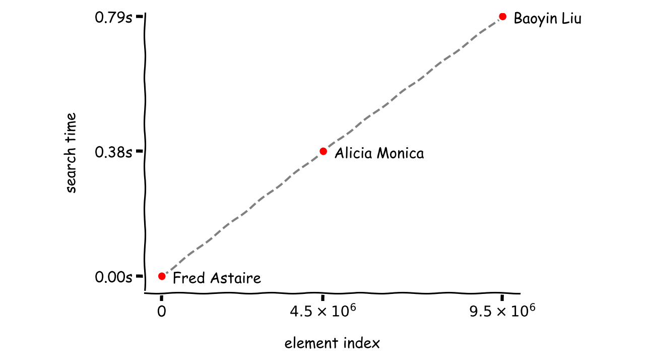
All samples lie on a straight line and can be described by a linear function, which is where the name of the algorithm comes from. You can assume that, on average, the time required to find any element using a linear search will be proportional to the number of all elements in the collection. They don’t scale well as the amount of data to search increases.
For example, biometric scanners available at some airports wouldn’t recognize passengers in a matter of seconds, had they been implemented using linear search. On the other hand, the linear search algorithm may be a good choice for smaller datasets, because it doesn’t require preprocessing the data. In such a case, the benefits of preprocessing wouldn’t pay back its cost.
Python already ships with linear search, so there’s no point in writing it yourself. The list data structure, for example, exposes a method that will return the index of an element or raise an exception otherwise:
>>> fruits = ['orange', 'plum', 'banana', 'apple']
>>> fruits.index('banana')
2
>>> fruits.index('blueberry')
Traceback (most recent call last):
  File "<stdin>", line 1, in <module>
ValueError: 'blueberry' is not in list
This can also tell you if the element is present in the collection, but a more Pythonic way would involve using the versatile in operator:
>>> 'banana' in fruits
True
>>> 'blueberry' in fruits
False
It’s worth noting that despite using linear search under the hood, these built-in functions and operators will blow your implementation out of the water. That’s because they were written in pure C, which compiles to native machine code. The standard Python interpreter is no match for it, no matter how hard you try.
A quick test with the timeit module reveals that the Python implementation might run almost ten times slower than the equivalent native one:
>>> import timeit
>>> from search.linear import contains
>>> fruits = ['orange', 'plum', 'banana', 'apple']
>>> timeit.timeit(lambda: contains(fruits, 'blueberry'))
1.8904765040024358
>>> timeit.timeit(lambda: 'blueberry' in fruits)
0.22473459799948614
However, for sufficiently large datasets, even the native code will hit its limits, and the only solution will be to rethink the algorithm.
Note: The in operator doesn’t always do a linear search. When you use it on a set, for example, it does a hash-based search instead. The operator can work with any iterable, including tuple, list, set, dict, and str. You can even support your custom classes with it by implementing the magic method .__contains__() to define the underlying logic.
In real-life scenarios, the linear search algorithm should usually be avoided. For example, there was a time I wasn’t able to register my cat at the vet clinic because their system kept crashing. The doctor told me he must eventually upgrade his computer because adding more records into the database makes it run slower and slower.
I remember thinking to myself at that point that the person who wrote that software clearly didn’t know about the binary search algorithm!
Binary Search
The word binary is generally associated with the number 2. In this context, it refers to dividing a collection of elements into two halves and throwing away one of them at each step of the algorithm. This can dramatically reduce the number of comparisons required to find an element. But there’s a catch—elements in the collection must be sorted first.
The idea behind it resembles the steps for finding a page in a book. At first, you typically open the book to a completely random page or at least one that’s close to where you think your desired page might be.
Occasionally, you’ll be fortunate enough to find that page on the first try. However, if the page number is too low, then you know the page must be to the right. If you overshoot on the next try, and the current page number is higher than the page you’re looking for, then you know for sure that it must be somewhere in between.
You repeat the process, but rather than choosing a page at random, you check the page located right in the middle of that new range. This minimizes the number of tries. A similar approach can be used in the number guessing game. If you haven’t heard of that game, then you can look it up on the Internet to get a plethora of examples implemented in Python.
Note: Sometimes, if the values are uniformly distributed, you can calculate the middle index with linear interpolation rather than taking the average. This variation of the algorithm will require even fewer steps.
The page numbers that restrict the range of pages to search through are known as the lower bound and the upper bound. In binary search, you commonly start with the first page as the lower bound and the last page as the upper bound. You must update both bounds as you go. For example, if the page you turn to is lower than the one you’re looking for, then that’s your new lower bound.
Let’s say you were looking for a strawberry in a collection of fruits sorted in ascending order by size:
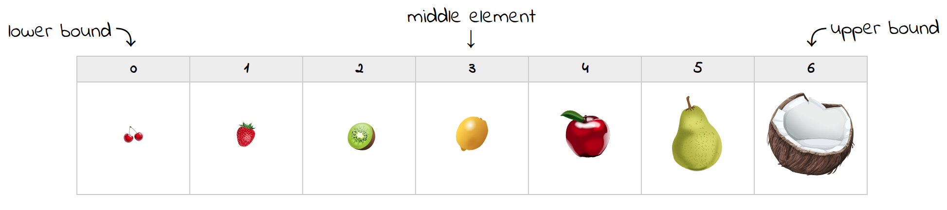
On the first attempt, the element in the middle happens to be a lemon. Since it’s bigger than a strawberry, you can discard all elements to the right, including the lemon. You’ll move the upper bound to a new position and update the middle index:
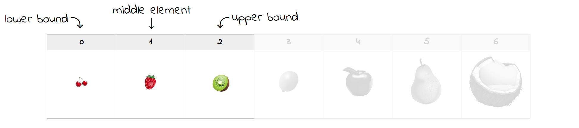
Now, you’re left with only half of the fruits you began with. The current middle element is indeed the strawberry you were looking for, which concludes the search. If it wasn’t, then you’d just update the bounds accordingly and continue until they pass each other. For example, looking for a missing plum, which would go between the strawberry and a kiwi, will end with the following result:

Notice there weren’t that many comparisons that had to be made in order to find the desired element. That’s the magic of binary search. Even if you’re dealing with a million elements, you’d only require at most a handful of checks. This number won’t exceed the logarithm base two of the total number of elements due to halving. In other words, the number of remaining elements is reduced by half at each step.
This is possible because the elements are already sorted by size. However, if you wanted to find fruits by another key, such as a color, then you’d have to sort the entire collection once again. To avoid the costly overhead of sorting, you might try to compute different views of the same collection in advance. This is somewhat similar to creating a database index.
Consider what happens if you add, delete or update an element in a collection. For a binary search to continue working, you’d need to maintain the proper sort order. This can be done with the bisect module, which you’ll read about in the upcoming section.
You’ll see how to implement the binary search algorithm in Python later on in this tutorial. For now, let’s confront it with the IMDb dataset. Notice that there are different people to search for than before. That’s because the dataset must be sorted for binary search, which reorders the elements. The new elements are located roughly at the same indices as before, to keep the measurements comparable:
| Search Term | Element Index | Average Time | Comparisons |
|---|---|---|---|
| (…) Berendse | 0 |
6.52µs |
23 |
| Jonathan Samuangte | 4,499,997 |
6.99µs |
24 |
| Yorgos Rahmatoulin | 9,500,001 |
6.5µs |
23 |
| missing | N/A |
7.2µs |
23 |
The answers are nearly instantaneous. In the average case, it takes only a few microseconds for the binary search to find one element among all nine million! Other than that, the number of comparisons for the chosen elements remains almost constant, which coincides with the following formula:

Finding most elements will require the highest number of comparisons, which can be derived from a logarithm of the size of the collection. Conversely, there’s just one element in the middle that can be found on the first try with one comparison.
Binary search is a great example of a divide-and-conquer technique, which partitions one problem into a bunch of smaller problems of the same kind. The individual solutions are then combined to form the final answer. Another well-known example of this technique is the Quicksort algorithm.
Note: Don’t confuse divide-and-conquer with dynamic programming, which is a somewhat similar technique.
Unlike other search algorithms, binary search can be used beyond just searching. For example, it allows for set membership testing, finding the largest or smallest value, finding the nearest neighbor of the target value, performing range queries, and more.
If speed is a top priority, then binary search is not always the best choice. There are even faster algorithms that can take advantage of hash-based data structures. However, those algorithms require a lot of additional memory, whereas binary search offers a good space-time tradeoff.
Hash-Based Search
To search faster, you need to narrow down the problem space. Binary search achieves that goal by halving the number of candidates at each step. That means that even if you have one million elements, it takes at most twenty comparisons to determine if the element is present, provided that all elements are sorted.
The fastest way to search is to know where to find what you’re looking for. If you knew the exact memory location of an element, then you’d access it directly without the need for searching in the first place. Mapping an element or (more commonly) one of its keys to the element location in memory is referred to as hashing.
You can think of hashing not as searching for the specific element, but instead computing the index based on the element itself. That’s the job of a hash function, which needs to hold certain mathematical properties. A good hash function should:
- Take arbitrary input and turn it into a fixed-size output.
- Have a uniform value distribution to mitigate hash collisions.
- Produce deterministic results.
- Be a one-way function.
- Amplify input changes to achieve the avalanche effect.
At the same time, it shouldn’t be too computationally expensive, or else its cost would outweigh the gains. A hash function is also used for data integrity verification as well as in cryptography.
A data structure that uses this concept to map keys into values is called a map, a hash table, a dictionary, or an associative array.
Note: Python has two built-in data structures, namely set and dict, which rely on the hash function to find elements. While a set hashes its elements, a dict uses the hash function against element keys. To find out exactly how a dict is implemented in Python, check out Raymond Hettinger’s conference talk on Modern Python Dictionaries.
Another way to visualize hashing is to imagine so-called buckets of similar elements grouped under their respective keys. For example, you may be harvesting fruits into different buckets based on color:

The coconut and a kiwi fruit go to the bucket labeled brown, while an apple ends up in a bucket with the red label, and so on. This allows you to glance through a fraction of the elements quickly. Ideally, you want to have only one fruit in each bucket. Otherwise, you get what’s known as a collision, which leads to extra work.
Note: The buckets, as well as their contents, are typically in no particular order.
Let’s put the names from the IMDb dataset into a dictionary, so that each name becomes a key, and the corresponding value becomes its index:
>>> from benchmark import load_names  # Sample code to download
>>> names = load_names('names.txt')
>>> index_by_name = {
...     name: index for index, name in enumerate(names)
... }
After loading textual names into a flat list, you can enumerate() it inside a dictionary comprehension to create the mapping. Now, checking the element’s presence as well as getting its index is straightforward:
>>> 'Guido van Rossum' in index_by_name
False
>>> 'Arnold Schwarzenegger' in index_by_name
True
>>> index_by_name['Arnold Schwarzenegger']
215
Thanks to the hash function used behind the scenes, you don’t have to implement any search at all!
Here’s how the hash-based search algorithm performs against the IMDb dataset:
| Search Term | Element Index | Best Time | Average Time | Worst Time |
|---|---|---|---|---|
| Fred Astaire | 0 |
0.18µs |
0.4µs |
1.9µs |
| Alicia Monica | 4,500,000 |
0.17µs |
0.4µs |
2.4µs |
| Baoyin Liu | 9,500,000 |
0.17µs |
0.4µs |
2.6µs |
| missing | N/A |
0.19µs |
0.4µs |
1.7µs |
Not only is the average time an order of magnitude faster than the already fast binary search Python implementation, but the speed is also sustained across all elements regardless of where they are.
The price for that gain is approximately 0.5 GB of more memory consumed by the Python process, slower load time, and the need to keep that additional data consistent with dictionary contents. In turn, the lookup is very quick, while updates and insertions are slightly slower when compared to a list.
Another constraint that dictionaries impose on their keys is that they must be hashable, and their hash values can’t change over time. You can check if a particular data type is hashable in Python by calling hash() on it:
>>> key = ['round', 'juicy']
>>> hash(key)
Traceback (most recent call last):
  File "<stdin>", line 1, in <module>
TypeError: unhashable type: 'list'
Mutable collections—such as a list, set, and dict—aren’t hashable. In practice, dictionary keys should be immutable because their hash value often depends on some attributes of the key. If a mutable collection was hashable and could be used as a key, then its hash value would be different every time the contents changed. Consider what would happen if a particular fruit changed color due to ripening. You’d be looking for it in the wrong bucket!
The hash function has many other uses. For example, it’s used in cryptography to avoid storing passwords in plain text form, as well as for data integrity verification.
Using the bisect Module
Binary search in Python can be performed using the built-in bisect module, which also helps with preserving a list in sorted order. It’s based on the bisection method for finding roots of functions. This module comes with six functions divided into two categories:
| Find Index | Insert Element |
|---|---|
bisect() |
insort() |
bisect_left() |
insort_left() |
bisect_right() |
insort_right() |
These functions allow you to either find an index of an element or add a new element in the right position. Those in the first row are just aliases for bisect_right() and insort_right(), respectively. In reality, you’re dealing with only four functions.
Note: It’s your responsibility to sort the list before passing it to one of the functions. If the elements aren’t sorted, then you’ll most likely get incorrect results.
Without further ado, let’s see the bisect module in action.
Finding an Element
To find the index of an existing element in a sorted list, you want to bisect_left():
>>> import bisect
>>> sorted_fruits = ['apple', 'banana', 'orange', 'plum']
>>> bisect.bisect_left(sorted_fruits, 'banana')
1
The output tells you that a banana is the second fruit on the list because it was found at index 1. However, if an element was missing, then you’d still get its expected position:
>>> bisect.bisect_left(sorted_fruits, 'apricot')
1
>>> bisect.bisect_left(sorted_fruits, 'watermelon')
4
Even though these fruits aren’t on the list yet, you can get an idea of where to put them. For example, an apricot should come between the apple and the banana, whereas a watermelon should become the last element. You’ll know if an element was found by evaluating two conditions:
-
Is the index within the size of the list?
-
Is the value of the element the desired one?
This can be translated to a universal function for finding elements by value:
def find_index(elements, value):
    index = bisect.bisect_left(elements, value)
    if index < len(elements) and elements[index] == value:
        return index
When there’s a match, the function will return the corresponding element index. Otherwise, it’ll return None implicitly.
To search by key, you have to maintain a separate list of keys. Since this incurs an additional cost, it’s worthwhile to calculate the keys up front and reuse them as much as possible. You can define a helper class to be able to search by different keys without introducing much code duplication:
class SearchBy:
    def __init__(self, key, elements):
        self.elements_by_key = sorted([(key(x), x) for x in elements])
        self.keys = [x[0] for x in self.elements_by_key]
The key is a function passed as the first parameter to __init__(). Once you have it, you make a sorted list of key-value pairs to be able to retrieve an element from its key at a later time. Representing pairs with tuples guarantees that the first element of each pair will be sorted. In the next step, you extract the keys to make a flat list that’s suitable for your binary search Python implementation.
Then there’s the actual method for finding elements by key:
class SearchBy:
    def __init__(self, key, elements):
        ...

    def find(self, value):
        index = bisect.bisect_left(self.keys, value)
        if index < len(self.keys) and self.keys[index] == value:
            return self.elements_by_key[index][1]
This code bisects the list of sorted keys to get the index of an element by key. If such a key exists, then its index can be used to get the corresponding pair from the previously computed list of key-value pairs. The second element of that pair is the desired value.
Note: This is just an illustrative example. You’ll be better off using the recommended recipe, which is mentioned in the official documentation.
If you had multiple bananas, then bisect_left() would return the leftmost instance:
>>> sorted_fruits = [
...     'apple',
...     'banana', 'banana', 'banana',
...     'orange',
...     'plum'
... ]
>>> bisect.bisect_left(sorted_fruits, 'banana')
1
Predictably, to get the rightmost banana, you’d need to call bisect_right() or its bisect() alias. However, those two functions return one index further from the actual rightmost banana, which is useful for finding the insertion point of a new element:
>>> bisect.bisect_right(sorted_fruits, 'banana')
4
>>> bisect.bisect(sorted_fruits, 'banana')
4
>>> sorted_fruits[4]
'orange'
When you combine the code, you can see how many bananas you have:
>>> l = bisect.bisect_left(sorted_fruits, 'banana')
>>> r = bisect.bisect_right(sorted_fruits, 'banana')
>>> r - l
3
If an element were missing, then both bisect_left() and bisect_right() would return the same index yielding zero bananas.
Inserting a New Element
Another practical application of the bisect module is maintaining the order of elements in an already sorted list. After all, you wouldn’t want to sort the whole list every time you had to insert something into it. In most cases, all three functions can be used interchangeably:
>>> import bisect
>>> sorted_fruits = ['apple', 'banana', 'orange']
>>> bisect.insort(sorted_fruits, 'apricot')
>>> bisect.insort_left(sorted_fruits, 'watermelon')
>>> bisect.insort_right(sorted_fruits, 'plum')
>>> sorted_fruits
['apple', 'apricot', 'banana', 'orange', 'plum', 'watermelon']
You won’t see any difference until there are duplicates in your list. But even then, it won’t become apparent as long as those duplicates are simple values. Adding another banana to the left will have the same effect as adding it to the right.
To notice the difference, you need a data type whose objects can have unique identities despite having equal values. Let’s define a Person type using the @dataclass decorator, which was introduced in Python 3.7:
from dataclasses import dataclass, field

@dataclass
class Person:
    name: str
    number: int = field(compare=False)

    def __repr__(self):
        return f'{self.name}({self.number})'
A person has a name and an arbitrary number assigned to it. By excluding the number field from the equality test, you make two people equal even if they have different values of that attribute:
>>> p1 = Person('John', 1)
>>> p2 = Person('John', 2)
>>> p1 == p2
True
On the other hand, those two variables refer to completely separate entities, which allows you to make a distinction between them:
>>> p1 is p2
False
>>> p1
John(1)
>>> p2
John(2)
The variables p1 and p2 are indeed different objects.
Note that instances of a data class aren’t comparable by default, which prevents you from using the bisection algorithm on them:
>>> alice, bob = Person('Alice', 1), Person('Bob', 1)
>>> alice < bob
Traceback (most recent call last):
  File "<stdin>", line 1, in <module>
TypeError: '<' not supported between instances of 'Person' and 'Person'
Python doesn’t know to order alice and bob, because they’re objects of a custom class. Traditionally, you’d implement the magic method .__lt__() in your class, which stands for less than, to tell the interpreter how to compare such elements. However, the @dataclass decorator accepts a few optional Boolean flags. One of them is order, which results in an automatic generation of the magic methods for comparison when set to True:
@dataclass(order=True)
class Person:
    ...
In turn, this allows you to compare two people and decide which one comes first:
>>> alice < bob
True
>>> bob < alice
False
Finally, you can take advantage of the name and number properties to observe where various functions insert new people to the list:
>>> sorted_people = [Person('John', 1)]
>>> bisect.insort_left(sorted_people, Person('John', 2))
>>> bisect.insort_right(sorted_people, Person('John', 3))
>>> sorted_people
[John(2), John(1), John(3)]
The numbers in parentheses after the names indicate the insertion order. In the beginning, there was just one John, who got the number 1. Then, you added its duplicate to the left, and later one more to the right.
Implementing Binary Search in Python
Keep in mind that you probably shouldn’t implement the algorithm unless you have a strong reason to. You’ll save time and won’t need to reinvent the wheel. The chances are that the library code is mature, already tested by real users in a production environment, and has extensive functionality delivered by multiple contributors.
That said, there are times when it makes sense to roll up your sleeves and do it yourself. Your company might have a policy banning certain open source libraries due to licensing or security matters. Maybe you can’t afford another dependency due to memory or network bandwidth constraints. Lastly, writing code yourself might be a great learning tool!
You can implement most algorithms in two ways:
- Iteratively
- Recursively
However, there are exceptions to that rule. One notable example is the Ackermann function, which can only be expressed in terms of recursion.
Before you go any further, make sure that you have a good grasp of the binary search algorithm. You can refer to an earlier part of this tutorial for a quick refresher.
Iteratively
The iterative version of the algorithm involves a loop, which will repeat some steps until the stopping condition is met. Let’s begin by implementing a function that will search elements by value and return their index:
def find_index(elements, value):
    ...
You’re going to reuse this function later.
Assuming that all elements are sorted, you can set the lower and the upper boundaries at the opposite ends of the sequence:
def find_index(elements, value):
    left, right = 0, len(elements) - 1
Now, you want to identify the middle element to see if it has the desired value. Calculating the middle index can be done by taking the average of both boundaries:
def find_index(elements, value):
    left, right = 0, len(elements) - 1
    middle = (left + right) // 2
Notice how an integer division helps to handle both an odd and even number of elements in the bounded range by flooring the result. Depending on how you’re going to update the boundaries and define the stopping condition, you could also use a ceiling function.
Next, you either finish or split the sequence in two and continue searching in one of the resultant halves:
def find_index(elements, value):
    left, right = 0, len(elements) - 1
    middle = (left + right) // 2

    if elements[middle] == value:
        return middle

    if elements[middle] < value:
        left = middle + 1
    elif elements[middle] > value:
        right = middle - 1
If the element in the middle was a match, then you return its index. Otherwise, if it was too small, then you need to move the lower boundary up. If it was too big, then you need to move the upper boundary down.
To keep going, you have to enclose most of the steps in a loop, which will stop when the lower boundary overtakes the upper one:
def find_index(elements, value):
    left, right = 0, len(elements) - 1

    while left <= right:
        middle = (left + right) // 2

        if elements[middle] == value:
            return middle

        if elements[middle] < value:
            left = middle + 1
        elif elements[middle] > value:
            right = middle - 1
In other words, you want to iterate as long as the lower boundary is below or equal to the upper one. Otherwise, there was no match, and the function returns None implicitly.
Searching by key boils down to looking at an object’s attributes instead of its literal value. A key could be the number of characters in a fruit’s name, for example. You can adapt find_index() to accept and use a key parameter:
def find_index(elements, value, key):
    left, right = 0, len(elements) - 1

    while left <= right:
        middle = (left + right) // 2
        middle_element = key(elements[middle])

        if middle_element == value:
            return middle

        if middle_element < value:
            left = middle + 1
        elif middle_element > value:
            right = middle - 1
However, you must also remember to sort the list using the same key that you’re going to search with:
>>> fruits = ['orange', 'plum', 'watermelon', 'apple']
>>> fruits.sort(key=len)
>>> fruits
['plum', 'apple', 'orange', 'watermelon']
>>> fruits[find_index(fruits, key=len, value=10)]
'watermelon'
>>> print(find_index(fruits, key=len, value=3))
None
In the example above, watermelon was chosen because its name is precisely ten characters long, while no fruits on the list have names made up of three letters.
That’s great, but at the same time, you’ve just lost the ability to search by value. To remedy this, you could assign the key a default value of None and then check if it was given or not. However, in a more streamlined solution, you’d always want to call the key. By default, it would be an identity function returning the element itself:
def identity(element):
    return element

def find_index(elements, value, key=identity):
    ...
Alternatively, you might define the identity function inline with an anonymous lambda expression:
def find_index(elements, value, key=lambda x: x):
    ...
find_index() answers only one question. There are still two others, which are “Is it there?” and “What is it?” To answer these two, you can build on top of it:
def find_index(elements, value, key):
    ...

def contains(elements, value, key=identity):
    return find_index(elements, value, key) is not None

def find(elements, value, key=identity):
    index = find_index(elements, value, key)
    return None if index is None else elements[index]
With these three functions, you can tell almost everything about an element. However, you still haven’t addressed duplicates in your implementation. What if you had a collection of people, and some of them shared a common name or surname? For example, there might be a Smith family or a few guys going by the name of John among the people:
people = [
    Person('Bob', 'Williams'),
    Person('John', 'Doe'),
    Person('Paul', 'Brown'),
    Person('Alice', 'Smith'),
    Person('John', 'Smith'),
]
To model the Person type, you can modify a data class defined earlier:
from dataclasses import dataclass

@dataclass(order=True)
class Person:
    name: str
    surname: str
Notice the use of the order attribute to enable automatic generation of magic methods for comparing instances of the class by all fields. Alternatively, you might prefer to take advantage of the namedtuple, which has a shorter syntax:
from collections import namedtuple
Person = namedtuple('Person', 'name surname')
Both definitions are fine and interchangeable. Each person has a name and a surname attribute. To sort and search by one of them, you can conveniently define the key function with an attrgetter() available in the built-in operator module:
>>> from operator import attrgetter
>>> by_surname = attrgetter('surname')
>>> people.sort(key=by_surname)
>>> people
[Person(name='Paul', surname='Brown'),
 Person(name='John', surname='Doe'),
 Person(name='Alice', surname='Smith'),
 Person(name='John', surname='Smith'),
 Person(name='Bob', surname='Williams')]
Notice how people are now sorted by surname in ascending order. There’s John Smith and Alice Smith, but binary searching for the Smith surname currently gives you only one arbitrary result:
>>> find(people, key=by_surname, value='Smith')
Person(name='Alice', surname='Smith')
To mimic the features of the bisect module shown before, you can write your own version of bisect_left() and bisect_right(). Before finding the leftmost instance of a duplicate element, you want to determine if there’s such an element at all:
def find_leftmost_index(elements, value, key=identity):
    index = find_index(elements, value, key)
    if index is not None:
        ...
    return index
If some index has been found, then you can look to the left and keep moving until you come across an element with a different key or there are no more elements:
def find_leftmost_index(elements, value, key=identity):
    index = find_index(elements, value, key)
    if index is not None:
        while index >= 0 and key(elements[index]) == value:
            index -= 1
        index += 1
    return index
Once you go past the leftmost element, you need to move the index back by one position to the right.
Finding the rightmost instance is quite similar, but you need to flip the conditions:
def find_rightmost_index(elements, value, key=identity):
    index = find_index(elements, value, key)
    if index is not None:
        while index < len(elements) and key(elements[index]) == value:
            index += 1
        index -= 1
    return index
Instead of going left, now you’re going to the right until the end of the list. Using both functions allows you to find all occurrences of duplicate items:
def find_all_indices(elements, value, key=identity):
    left = find_leftmost_index(elements, value, key)
    right = find_rightmost_index(elements, value, key)
    if left and right:
        return set(range(left, right + 1))
    return set()
This function always returns a set. If the element isn’t found, then the set will be empty. If the element is unique, then the set will be made up of only a single index. Otherwise, there will be multiple indices in the set.
To wrap up, you can define even more abstract functions to complete your binary search Python library:
def find_leftmost(elements, value, key=identity):
    index = find_leftmost_index(elements, value, key)
    return None if index is None else elements[index]

def find_rightmost(elements, value, key=identity):
    index = find_rightmost_index(elements, value, key)
    return None if index is None else elements[index]

def find_all(elements, value, key=identity):
    return {elements[i] for i in find_all_indices(elements, value, key)}
Not only does this allow you to pinpoint the exact location of elements on the list, but also to retrieve those elements. You’re able to ask very specific questions:
| Is it there? | Where is it? | What is it? |
|---|---|---|
contains() |
find_index() |
find() |
find_leftmost_index() |
find_leftmost() |
|
find_rightmost_index() |
find_rightmost() |
|
find_all_indices() |
find_all() |
The complete code of this binary search Python library can be found at the link below:
Get Sample Code: Click here to get the sample code you’ll use to learn about binary search in Python in this tutorial.
Recursively
For the sake of simplicity, you’re only going to consider the recursive version of contains(), which tells you if an element was found.
Note: My favorite definition of recursion was given in an episode of the Fun Fun Function series about functional programming in JavaScript:
“Recursion is when a function calls itself until it doesn’t.”
— Mattias Petter Johansson
The most straightforward approach would be to take the iterative version of binary search and use the slicing operator to chop the list:
def contains(elements, value):
    left, right = 0, len(elements) - 1

    if left <= right:
        middle = (left + right) // 2

        if elements[middle] == value:
            return True

        if elements[middle] < value:
            return contains(elements[middle + 1:], value)
        elif elements[middle] > value:
            return contains(elements[:middle], value)

    return False
Instead of looping, you check the condition once and sometimes call the same function on a smaller list. What could go wrong with that? Well, it turns out that slicing generates copies of element references, which can have noticeable memory and computational overhead.
To avoid copying, you might reuse the same list but pass different boundaries into the function whenever necessary:
def contains(elements, value, left, right):
    if left <= right:
        middle = (left + right) // 2

        if elements[middle] == value:
            return True

        if elements[middle] < value:
            return contains(elements, value, middle + 1, right)
        elif elements[middle] > value:
            return contains(elements, value, left, middle - 1)

    return False
The downside is that every time you want to call that function, you have to pass initial boundaries, making sure they’re correct:
>>> sorted_fruits = ['apple', 'banana', 'orange', 'plum']
>>> contains(sorted_fruits, 'apple', 0, len(sorted_fruits) - 1)
True
If you were to make a mistake, then it would potentially not find that element. You can improve this by using default function arguments or by introducing a helper function that delegates to the recursive one:
def contains(elements, value):
    return recursive(elements, value, 0, len(elements) - 1)

def recursive(elements, value, left, right):
    ...
Going further, you might prefer to nest one function in another to hide the technical details and to take advantage of variable reuse from outer scope:
def contains(elements, value):
    def recursive(left, right):
        if left <= right:
            middle = (left + right) // 2
            if elements[middle] == value:
                return True
            if elements[middle] < value:
                return recursive(middle + 1, right)
            elif elements[middle] > value:
                return recursive(left, middle - 1)
        return False
    return recursive(0, len(elements) - 1)
The recursive() inner function can access both elements and value parameters even though they’re defined in the enclosing scope. The life cycle and visibility of variables in Python is dictated by the so-called LEGB rule, which tells the interpreter to look for symbols in the following order:
- Local scope
- Enclosing scope
- Global scope
- Built-in symbols
This allows variables that are defined in outer scope to be accessed from within nested blocks of code.
The choice between an iterative and a recursive implementation is often the net result of performance considerations, convenience, as well as personal taste. However, there are also certain risks involved with recursion, which is one of the subjects of the next section.
Covering Tricky Details
Here’s what the author of The Art of Computer Programming has to say about implementing the binary search algorithm:
“Although the basic idea of binary search is comparatively straightforward, the details can be surprisingly tricky, and many good programmers have done it wrong the first few times they tried.”
— Donald Knuth
If that doesn’t deter you enough from the idea of writing the algorithm yourself, then maybe this will. The standard library in Java had a subtle bug in their implementation of binary search, which remained undiscovered for a decade! But the bug itself traces its roots much earlier than that.
Note: I once fell victim to the binary search algorithm during a technical screening. There were a couple of coding puzzles to solve, including a binary search one. Guess which one I failed to complete? Yeah.
The following list isn’t exhaustive, but at the same time, it doesn’t talk about common mistakes like forgetting to sort the list.
Integer Overflow
This is the Java bug that was just mentioned. If you recall, the binary search Python algorithm inspects the middle element of a bounded range in a sorted collection. But how is that middle element chosen exactly? Usually, you take the average of the lower and upper boundary to find the middle index:
middle = (left + right) // 2
This method of calculating the average works just fine in the overwhelming majority of cases. However, once the collection of elements becomes sufficiently large, the sum of both boundaries won’t fit the integer data type. It’ll be larger than the maximum value allowed for integers.
Some programming languages might raise an error in such situations, which would immediately stop program execution. Unfortunately, that’s not always the case. For example, Java silently ignores this problem, letting the value flip around and become some seemingly random number. You’ll only know about the problem as long as the resulting number happens to be negative, which throws an IndexOutOfBoundsException.
Here’s an example that demonstrates this behavior in jshell, which is kind of like an interactive interpreter for Java:
jshell> var a = Integer.MAX_VALUE
a ==> 2147483647

jshell> a + 1
$2 ==> -2147483648
A safer way to find the middle index could be calculating the offset first and then adding it to the lower boundary:
middle = left + (right - left) // 2
Even if both values are maxed out, the sum in the formula above will never be. There are a few more ways, but the good news is that you don’t need to worry about any of these, because Python is free from the integer overflow error. There’s no upper limit on how big integers can be other than your memory:
>>> 2147483647**7
210624582650556372047028295576838759252690170086892944262392971263
However, there’s a catch. When you call functions from a library, that code might be subject to the C language constraints and still cause an overflow. There are plenty of libraries based on the C language in Python. You could even build your own C extension module or load a dynamically-linked library into Python using ctypes.
Stack Overflow
The stack overflow problem may, theoretically, concern the recursive implementation of binary search. Most programming languages impose a limit on the number of nested function calls. Each call is associated with a return address stored on a stack. In Python, the default limit is a few thousand levels of such calls:
>>> import sys
>>> sys.getrecursionlimit()
1000
This won’t be enough for a lot of recursive functions. However, it’s very unlikely that a binary search in Python would ever need more due to its logarithmic nature. You’d need a collection of two to the power of three thousand elements. That’s a number with over nine hundred digits!
Nevertheless, it’s still possible for the infinite recursion error to arise if the stopping condition is stated incorrectly due to a bug. In such a case, the infinite recursion will eventually cause a stack overflow.
Note: The stack overflow error is very common among languages with manual memory management. People would often google those errors to see if someone else already had similar issues, which gave the name to a popular Q&A site for programmers.
You can temporarily lift or decrease the recursion limit to simulate a stack overflow error. Note that the effective limit will be smaller because of the functions that the Python runtime environment has to call:
>>> def countup(limit, n=1):
...     print(n)
...     if n < limit:
...         countup(limit, n + 1)
...
>>> import sys
>>> sys.setrecursionlimit(7)  # Actual limit is 3
>>> countup(10)
1
2
3
Traceback (most recent call last):
  File "<stdin>", line 1, in <module>
  File "<stdin>", line 4, in countup
  File "<stdin>", line 4, in countup
  File "<stdin>", line 2, in countup
RecursionError: maximum recursion depth exceeded while calling a Python object
The recursive function was called three times before saturating the stack. The remaining four calls must have been made by the interactive interpreter. If you run that same code in PyCharm or an alternative Python shell, then you might get a different result.
Duplicate Elements
You’re aware of the possibility of having duplicate elements in the list and you know how to deal with them. This is just to emphasize that a conventional binary search in Python might not produce deterministic results. Depending on how the list was sorted or how many elements it has, you’ll get a different answer:
>>> from search.binary import *
>>> sorted_fruits = ['apple', 'banana', 'banana', 'orange']
>>> find_index(sorted_fruits, 'banana')
1
>>> sorted_fruits.append('plum')
>>> find_index(sorted_fruits, 'banana')
2
There are two bananas on the list. At first, the call to find_index() returns the left one. However, adding a completely unrelated element at the end of the list makes the same call give you a different banana.
The same principle, known as algorithm stability, applies to sorting algorithms. Some are stable, meaning they don’t change the relative positions of equivalent elements. Others don’t make such guarantees. If you ever need to sort elements by multiple criteria, then you should always start from the least significant key to retain stability.
Floating-Point Rounding
So far you’ve only searched for fruits or people, but what about numbers? They should be no different, right? Let’s make a list of floating-point numbers at 0.1 increments using a list comprehension:
>>> sorted_numbers = [0.1*i for i in range(1, 4)]
The list should contain numbers the one-tenth, two-tenths, and three-tenths. Surprisingly, only two of those three numbers can be found:
>>> from search.binary import contains
>>> contains(sorted_numbers, 0.1)
True
>>> contains(sorted_numbers, 0.2)
True
>>> contains(sorted_numbers, 0.3)
False
This isn’t a problem strictly related to binary search in Python, as the built-in linear search is consistent with it:
>>> 0.1 in sorted_numbers
True
>>> 0.2 in sorted_numbers
True
>>> 0.3 in sorted_numbers
False
It’s not even a problem related to Python but rather to how floating-point numbers are represented in computer memory. This is defined by the IEEE 754 standard for floating-point arithmetic. Without going into much detail, some decimal numbers don’t have a finite representation in binary form. Because of limited memory, those numbers get rounded, causing a floating-point rounding error.
Note: If you require maximum precision, then steer away from floating-point numbers. They’re great for engineering purposes. However, for monetary operations, you don’t want rounding errors to accumulate. It’s recommended to scale down all prices and amounts to the smallest unit, such as cents or pennies, and treat them as integers.
Alternatively, many programming languages have support for fixed-point numbers, such as the decimal type in Python. This puts you in control of when and how rounding is taking place.
If you do need to work with floating-point numbers, then you should replace exact matching with an approximate comparison. Let’s consider two variables with slightly different values:
>>> a = 0.3
>>> b = 0.1 * 3
>>> b
0.30000000000000004
>>> a == b
False
Regular comparison gives a negative result, although both values are nearly identical. Fortunately, Python comes with a function that will test if two values are close to each other within some small neighborhood:
>>> import math
>>> math.isclose(a, b)
True
That neighborhood, which is the maximum distance between the values, can be adjusted if needed:
>>> math.isclose(a, b, rel_tol=1e-16)
False
You can use that function to do a binary search in Python in the following way:
import math

def find_index(elements, value):
    left, right = 0, len(elements) - 1

    while left <= right:
        middle = (left + right) // 2

        if math.isclose(elements[middle], value):
            return middle

        if elements[middle] < value:
            left = middle + 1
        elif elements[middle] > value:
            right = middle - 1
On the other hand, this implementation of binary search in Python is specific to floating-point numbers only. You couldn’t use it to search for anything else without getting an error.
Analyzing the Time-Space Complexity of Binary Search
The following section will contain no code and some math concepts.
In computing, you can optimize the performance of pretty much any algorithm at the expense of increased memory use. For instance, you saw that a hash-based search of the IMDb dataset required an extra 0.5 GB of memory to achieve unparalleled speed.
Conversely, to save bandwidth, you’d compress a video stream before sending it over the network, increasing the amount of work to be done. This phenomenon is known as the space-time tradeoff and is useful in evaluating an algorithm’s complexity.
Time-Space Complexity
The computational complexity is a relative measure of how many resources an algorithm needs to do its job. The resources include computation time as well as the amount of memory it uses. Comparing the complexity of various algorithms allows you to make an informed decision about which is better in a given situation.
Note: Algorithms that don’t need to allocate more memory than their input data already consumes are called in-place, or in-situ, algorithms. This results in mutating the original data, which sometimes may have unwanted side-effects.
You looked at a few search algorithms and their average performance against a large dataset. It’s clear from those measurements that a binary search is faster than a linear search. You can even tell by what factor.
However, if you took the same measurements in a different environment, you’d probably get slightly or perhaps entirely different results. There are invisible factors at play that can be influencing your test. Besides, such measurements aren’t always feasible. So, how can you compare time complexities quickly and objectively?
The first step is to break down the algorithm into smaller pieces and find the one that is doing the most work. It’s likely going to be some elementary operation that gets called a lot and consistently takes about the same time to run. For search algorithms, such an operation might be the comparison of two elements.
Having established that, you can now analyze the algorithm. To find the time complexity, you want to describe the relationship between the number of elementary operations executed versus the size of the input. Formally, such a relationship is a mathematical function. However, you’re not interested in looking for its exact algebraic formula but rather estimating its overall shape.
There are a few well-known classes of functions that most algorithms fit in. Once you classify an algorithm according to one of them, you can put it on a scale:

These classes tell you how the number of elementary operations increases with the growing size of the input. They are, from left to right:
- Constant
- Logarithmic
- Linear
- Quasilinear
- Quadratic
- Exponential
- Factorial
This can give you an idea about the performance of the algorithm you’re considering. A constant complexity, regardless of the input size, is the most desired one. A logarithmic complexity is still pretty good, indicating a divide-and-conquer technique at use. The further to the right on this scale, the worse the complexity of the algorithm, because it has more work to do.
When you’re talking about the time complexity, what you typically mean is the asymptotic complexity, which describes the behavior under very large data sets. This simplifies the function formula by eliminating all terms and coefficients but the one that grows at the fastest rate (for example, n squared).
However, a single function doesn’t provide enough information to compare two algorithms accurately. The time complexity may vary depending on the volume of data. For example, the binary search algorithm is like a turbocharged engine, which builds pressure before it’s ready to deliver power. On the other hand, the linear search algorithm is fast from the start but quickly reaches its peak power and ultimately loses the race:
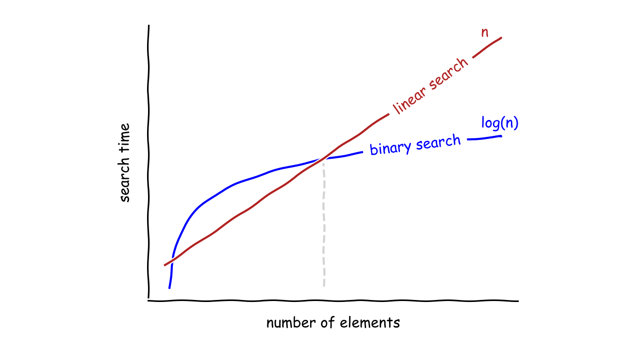
In terms of speed, the binary search algorithm starts to overtake the linear search when there’s a certain number of elements in the collection. For smaller collections, a linear search might be a better choice.
Note: Note that the same algorithm may have different optimistic, pessimistic, and average time complexity. For example, in the best-case scenario, a linear search algorithm will find the element at the first index, after running just one comparison.
On the other end of the spectrum, it’ll have to compare a reference value to all elements in the collection. In practice, you want to know the pessimistic complexity of an algorithm.
There are a few mathematical notations of the asymptotic complexity, which are used to compare algorithms. By far the most popular one is the Big O notation.
The Big O Notation
The Big O notation represents the worst-case scenario of asymptotic complexity. Although this might sound rather intimidating, you don’t need to know the formal definition. Intuitively, it’s a very rough measure of the rate of growth at the tail of the function that describes the complexity. You pronounce it as “big oh” of something:

That “something” is usually a function of data size or just the digit “one” that stands for a constant. For example, the linear search algorithm has a time complexity of O(n), while a hash-based search has O(1) complexity.
Note: When you say that some algorithm has complexity O(f(n)), where n is the size of the input data, then it means that the function f(n) is an upper bound of the graph of that complexity. In other words, the actual complexity of that algorithm won’t grow faster than f(n) multiplied by some constant, when n approaches infinity.
In real-life, the Big O notation is used less formally as both an upper and a lower bound. This is useful for the classification and comparison of algorithms without having to worry about the exact function formulas.
The Complexity of Binary Search
You’ll estimate the asymptotic time complexity of binary search by determining the number of comparisons in the worst-case scenario—when an element is missing—as a function of input size. You can approach this problem in three different ways:
- Tabular
- Graphical
- Analytical
The tabular method is about collecting empirical data, putting it in a table, and trying to guess the formula by eyeballing sampled values:
| Number of Elements | Number of Comparisons |
|---|---|
| 0 | 0 |
| 1 | 1 |
| 2 | 2 |
| 3 | 2 |
| 4 | 3 |
| 5 | 3 |
| 6 | 3 |
| 7 | 3 |
| 8 | 4 |
The number of comparisons grows as you increase the number of elements in the collection, but the rate of growth is slower than if it was a linear function. That’s an indication of a good algorithm that can scale with data.
If that doesn’t help you, you can try the graphical method, which visualizes the sampled data by drawing a graph:
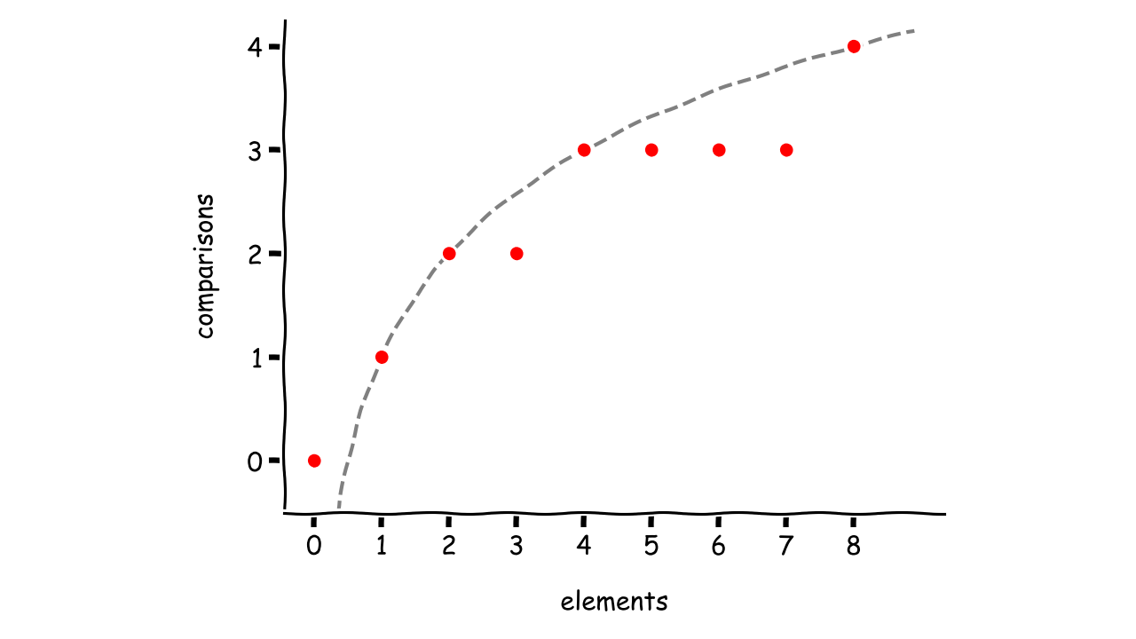
The data points seem to overlay with a curve, but you don’t have enough information to provide a conclusive answer. It could be a polynomial, whose graph turns up and down for larger inputs.
Taking the analytical approach, you can choose some relationship and look for patterns. For example, you might study how the number of elements shrinks in each step of the algorithm:
| Comparison | Number of Elements |
|---|---|
| - | n |
| 1st | n/2 |
| 2nd | n/4 |
| 3rd | n/8 |
| ⋮ | ⋮ |
| k-th | n/2 k |
In the beginning, you start with the whole collection of n elements. After the first comparison, you’re left with only half of them. Next, you have a quarter, and so on. The pattern that arises from this observation is that after k-th comparison, there are n/2 k elements. Variable k is the expected number of elementary operations.
After all k comparisons, there will be no more elements left. However, when you take one step back, that is k - 1, there will be exactly one element left. This gives you a convenient equation:

Multiply both sides of the equation by the denominator, then take the logarithm base two of the result, and move the remaining constant to the right. You’ve just found the formula for the binary search complexity, which is on the order of O(log(n)).
Conclusion
Now you know the binary search algorithm inside and out. You can flawlessly implement it yourself, or take advantage of the standard library in Python. Having tapped into the concept of time-space complexity, you’re able to choose the best search algorithm for the given situation.
Now you can:
- Use the
bisectmodule to do a binary search in Python - Implement binary search in Python recursively and iteratively
- Recognize and fix defects in a binary search Python implementation
- Analyze the time-space complexity of the binary search algorithm
- Search even faster than binary search
With all this knowledge, you’ll rock your programming interview! Whether the binary search algorithm is an optimal solution to a particular problem, you have the tools to figure it out on your own. You don’t need a computer science degree to do so.
You can grab all of the code you’ve seen in this tutorial at the link below:
Get Sample Code: Click here to get the sample code you’ll use to learn about binary search in Python in this tutorial.