Polars and pandas both provide DataFrame-based data analysis in Python, but they differ in syntax, performance, and features. In this tutorial on Polars vs pandas, you’ll compare their method chaining styles, run timed performance tests, explore LazyFrame optimizations in Polars, convert data between the two libraries, and create plots with their built-in tools. You’ll also examine scenarios where each library’s strengths make it the better choice.
By the end of this tutorial, you’ll understand that:
- Polars expressions and contexts let you build clear, optimized query pipelines without mutating your original data.
- LazyFrames with query optimization in Polars can outperform pandas for grouped and aggregated workloads.
- Streaming in Polars enables processing datasets that don’t fit in memory, which pandas can’t handle natively.
.to_pandas()andfrom_pandas()let you convert between DataFrame formats, and Narwhals offers a library-agnostic API.- Built-in plotting uses Altair for Polars and Matplotlib for pandas, allowing quick visualization directly from DataFrames.
To get the most out of this tutorial, it’s recommended that you already have a basic understanding of how to work with both pandas and Polars DataFrames, as well as Polars LazyFrames.
To complete the examples in this tutorial, you’ll use various tools and the Python REPL. You’ll use the command line to run some scripts that time your code and reveal how pandas and Polars compare. You’ll also take advantage of the plotting capabilities of Jupyter Notebook.
Much of the data you’ll use will be random and self-generated. You’ll also use a cleansed and reformatted Apache Parquet version of some freely available retail data from the UC Irvine Machine Learning Repository. Parquet files are optimized to store data and analyze it efficiently. This enables you to achieve optimal performance from the pandas and Polars libraries.
Before you start, you should download the online_retail.parquet file from the tutorial downloadables and place it into your project directory.
You’ll need to install the pandas and Polars libraries, as well as PyArrow, Matplotlib, Vega-Altair, and Narwhals, to make sure your code has everything it needs to run. You’ll also use NumPy, which is currently installed automatically when you install pandas.
You may also want to consider creating your own virtual environment within your project folder to install the necessary libraries. This will prevent them from interfering with your current setup.
You can install the required libraries using these commands at your command prompt:
$ python -m pip install polars \
                        pandas \
                        pyarrow \
                        narwhals \
                        altair \
                        jupyterlab \
                        matplotlib
All the code examples are provided in the downloadable materials for this tutorial, which you can download by clicking the link below:
Get Your Code: Click here to download the free sample code you’ll use to learn the differences between Polars and pandas.
Now that you’re set up, it’s time to get started and learn about the main differences between Polars and pandas.
Take the Quiz: Test your knowledge with our interactive “Polars vs pandas: What's the Difference?” quiz. You’ll receive a score upon completion to help you track your learning progress:

Interactive Quiz
Polars vs pandas: What's the Difference?Take this quiz to test your knowledge of the Polars vs pandas tutorial and review the key differences between these open-source Python libraries.
Do Polars and pandas Use the Same Syntax?
There are similarities between Polars and pandas. For example, they both support Series and DataFrames and can perform many of the same data analysis computations. However, there are some differences in their syntax.
To explore this, you’ll use the order details in your online_retail.parquet file to analyze both pandas and Polars DataFrames. This file contains the following data:
| Column Name | Description |
|---|---|
| InvoiceNo | Invoice number |
| StockCode | Stock code of item |
| Description | Item description |
| Quantity | Quantity purchased |
| InvoiceDate | Date invoiced |
| UnitPrice | Item price |
| CustomerID | Customer identifier |
| Country | Country of purchase made |
Next, you’ll analyze some of this data with pandas and then with Polars.
Using Index-Based Syntax in pandas
Suppose you want a DataFrame with a new Total column that contains the total cost of each purchase. You also want to apply filtering so you can concentrate on specific data.
To achieve this, you might write the following pandas code in your REPL:
pandas_polars_demo.py
>>> import pandas as pd

>>> orders_pandas = pd.read_parquet("online_retail.parquet")

>>> orders_pandas["Total"] = (
...     orders_pandas["Quantity"] * orders_pandas["UnitPrice"]
... )

>>> orders_pandas[["InvoiceNo", "Quantity", "UnitPrice", "Total"]][
...     orders_pandas["Total"] > 100
... ].head(3)
    InvoiceNo  Quantity  UnitPrice  Total
46     536371        80       2.55  204.0
65     536374        32      10.95  350.4
82     536376        48       3.45  165.6
This code uses pandas index-based syntax, inspired by NumPy, on which pandas was originally built. First, you add a new Total column to your DataFrame. The column is calculated by multiplying the values of the Quantity and UnitPrice columns together. This operation permanently changes your original DataFrame.
Next, you index the DataFrame using a list containing the four columns you want to see. You use the square-bracket notation ([]) in pandas for indexing, which is standard across the Python ecosystem. You then use the square brackets again, but this time to apply a filter so that only rows with totals greater than $100 are displayed. Finally, for brevity, you use .head(3) to restrict the output to the first three records.
This approach to writing pandas code mutates the DataFrame during processing. Once you’ve added the Total column, it becomes a permanent part of your DataFrame. If you make several such changes, your code can become difficult to follow, and the changes to the DataFrame become difficult to track. Also, your starting point for further processing is the updated DataFrame, which you may not always want.
Additionally, you can’t merge your code into a single operation since the Total column wouldn’t be recognized when you select it for display or filtering. That’s why you need a second operation to complete your analysis.
Using Method-Chaining Syntax in pandas
In addition to its index-based syntax, pandas also supports method chaining. This syntax allows you to specify multiple steps in a single operation and provides a clear audit trail of what happens to your DataFrame during its analysis.
You can rewrite the code above using method chaining. You need to read the data from the Parquet file and assign it to orders_pandas again:
pandas_polars_demo.py
>>> orders_pandas = pd.read_parquet("online_retail.parquet")

>>> (
...     orders_pandas
...     .assign(Total=orders_pandas["Quantity"] * orders_pandas["UnitPrice"])
...     .filter(["InvoiceNo", "Quantity", "UnitPrice", "Total"])
...     .query("Total > 100")
... ).head(3)
    InvoiceNo  Quantity  UnitPrice  Total
46     536371        80       2.55  204.0
65     536374        32      10.95  350.4
82     536376        48       3.45  165.6
Method chaining works because each method call, or link in the chain, returns a new DataFrame.
When you take your original orders_pandas DataFrame and apply .assign(Total=orders_pandas["Quantity"] * orders_pandas["UnitPrice"]) to it, you get a new DataFrame with a new Total column containing the product of the Quantity and UnitPrice columns. The original orders_pandas DataFrame remains unchanged.
Then, when you apply .filter() to this new DataFrame, you create an updated DataFrame containing only the four columns: InvoiceNo, Quantity, UnitPrice, and Total. This operation recognizes the Total column since you apply .filter() to the DataFrame that .assign() returns.
Finally, you use .query() to restrict the rows output to only those with values greater than one hundred in their Total column. It’s this final version of the DataFrame that contains your results. The intermediate versions created by each link in the chain have all been overwritten and the original orders_pandas hasn’t changed.
As in the previous example, you use .head(3) to restrict the output to the first three rows. You can add .head() directly to the chain of methods, but as it’s not part of the analysis, you can also add it at the end of the expression as shown above.
Note: There’s growing support for using method chaining in pandas. This syntax makes the code more readable and easier to maintain. Additionally, if you make an error, your original DataFrame won’t be altered.
Chaining also simplifies removing a link from your code. Removing one or more links won’t break the chain.
Suppose you sometimes need to run the previous analysis without the query. To do this, you can comment this part out:
>>> (
...     orders_pandas
...     .assign(Total=orders_pandas["Quantity"] * orders_pandas["UnitPrice"])
...     .filter(["InvoiceNo", "Quantity", "UnitPrice", "Total"])
... #   .query("Total > 100")
... ).head(3)
   InvoiceNo  Quantity  UnitPrice  Total
0     536365         6       2.55   15.3
1     536365         6       3.39  20.34
2     536365         8       2.75   22.0
This time, the .query() method is ignored. However, everything else runs as expected.
If you want to see more examples of method chaining in pandas, then be sure to check out the examples in Using Python for Data Analysis.
Using Method-Chaining Syntax in Polars
Polars syntax was designed with method chaining in mind. Here’s the same analysis you performed earlier, but this time using Polars. You’ll notice some differences from the pandas example shown above:
pandas_polars_demo.py
>>> import polars as pl

>>> orders_polars = pl.read_parquet("online_retail.parquet")

>>> (
...     orders_polars.select(
...         pl.col(["InvoiceNo", "Quantity", "UnitPrice"]),
...         Total=pl.col("Quantity") * pl.col("UnitPrice"),
...     ).filter(pl.col("Total") > 100)
... ).head(3)
shape: (3, 4)
┌───────────┬──────────┬───────────┬───────┐
│ InvoiceNo ┆ Quantity ┆ UnitPrice ┆ Total │
│ ---       ┆ ---      ┆ ---       ┆ ---   │
│ i64       ┆ i64      ┆ f64       ┆ f64   │
╞═══════════╪══════════╪═══════════╪═══════╡
│ 536371    ┆ 80       ┆ 2.55      ┆ 204.0 │
│ 536374    ┆ 32       ┆ 10.95     ┆ 350.4 │
│ 536376    ┆ 48       ┆ 3.45      ┆ 165.6 │
└───────────┴──────────┴───────────┴───────┘
When you write Polars code, you create it using expressions and contexts. In Polars, you use an expression to represent data or use it in a calculation. For example, pl.col("Quantity") * pl.col("UnitPrice") will instruct Polars to multiply together the "Quantity" and "UnitPrice" values from each column in a DataFrame.
To use your expressions productively, you need to put them into contexts. For example, expressions within the .select() context allow you to view specific columns, while those within the .filter() context enable you to restrict your output to only what you need.
Here you use the .select() context to choose the columns you want to see and to create and display the new Total column. You then use the .filter() context to apply your filter. The result is achieved in a single operation. As with the pandas chaining code you saw earlier, the original orders_polars DataFrame never changes.
Chaining creates code that can be more readable and maintainable. While pandas’ index-based syntax may feel intuitive for programmers familiar with NumPy, method chaining is often easier for beginners to learn.
Syntax differences aside, both pandas and Polars produce the same results, so you might think they both do the same thing behind the scenes. Read on and you’ll soon realize that they don’t.
What Are the Differences in Query Execution Between Polars vs pandas?
To understand how query execution differs between Polars and pandas, you need to consider not only their DataFrames but also Polars LazyFrames. In this section, you’ll create a pandas DataFrame, a Polars DataFrame, and a Polars LazyFrame to compare their data analysis capabilities.
Creating a Data Generation Script
To compare the time performance for pandas and Polars, you’ll create a Python script that can generate different quantities of data.
Create a new file in your project folder and name it data_generation.py, then add the following code to your file:
data_generation.py
import numpy as np

def generate_data(number_of_rows):
    rng = np.random.default_rng()

    return {
        "order_id": range(1, number_of_rows + 1),
        "region": rng.choice(
            ["North", "South", "East", "West"], size=number_of_rows
        ),
        "sales_person": rng.choice(
            ["Armstrong", "Aldrin", "Collins"], size=number_of_rows
        ),
        "product": rng.choice(
            ["Helmet", "Oxygen", "Boots", "Gloves"], size=number_of_rows
        ),
        "sales_income": rng.integers(1, 5001, size=number_of_rows),
    }
You use the NumPy library in this code, which was installed when you installed pandas. However, if you’re using NumPy in a different Python environment, you’ll need to install it separately.
Your script produces a Python dictionary that you’ll use to populate DataFrames. When you call generate_data(), you pass it the number of rows you want your DataFrame to have. Then, when you create a DataFrame with the dictionary returned by generate_data(), it’ll contain five columns and the number of rows you specified, each filled with random data.
Timing Operations Using DataFrames and LazyFrames
To see how well pandas DataFrames perform against both Polars DataFrames and LazyFrames, you’ll time a grouping operation. In this example, you’ll measure how long it takes to work out the total sales income for each salesperson within each product, within each region, using data generated with the generate_data() function you created earlier.
To begin, you’ll write a script to time your analysis. To keep the tests fair, you’ll make sure each one runs against the same data.
Importing the Libraries
Create a new file named benchmark.py, then add the following code:
benchmark.py
import functools
import sys
from timeit import Timer

import pandas as pd
import polars as pl

from data_generation import generate_data
You start by importing the built-in functools and sys modules.
The functools module provides you with various higher-order functions, which are functions that allow you to pass other functions to them as parameters.
The sys module allows you to pass command-line arguments to your script, which gives you more control over how it runs.
The timeit module enables you to measure the execution time of your code to determine its speed. This allows you to compare the performance between pandas and Polars. You’ll use a Timer object to do this.
You also import the pandas and polars libraries, as well as the generate_data() function you created earlier.
Creating the Functions to Be Tested
Next, add in three functions that will create a pandas DataFrame, a Polars DataFrame, and a Polars LazyFrame:
benchmark.py
# ...

def create_pandas_dataframe(test_data):
    return pd.DataFrame(test_data).convert_dtypes(dtype_backend="pyarrow")

def create_polars_dataframe(test_data):
    return pl.DataFrame(test_data)

def create_polars_lazyframe(test_data):
    return pl.LazyFrame(test_data)
Each function has a test_data parameter. You’ll pass the Python dictionary returned by generate_data() to these functions, and this is used to create the DataFrames and LazyFrames used in the time analysis. Each function returns the appropriate object. You also use .convert_dtypes() to ensure pandas uses the PyArrow data types instead of its default NumPy versions, since this newer backend is more performant.
Note: The NumPy data types will be removed from pandas version 3 and replaced with the more efficient PyArrow types. The explicit conversion won’t be needed when this happens.
Next, you create three more functions, each of which will perform the identical data analysis that you’ll time:
benchmark.py
# ...

def analyze_pandas_dataframe(pandas_df):
    return pandas_df.groupby(["region", "product", "sales_person"])[
        "sales_income"
    ].sum()

def analyze_polars_dataframe(polars_df):
    return polars_df.group_by(["region", "product", "sales_person"]).agg(
        total_sales=pl.col("sales_income").sum()
    )

def analyze_polars_lazyframe(polars_lf):
    return polars_lf.group_by(["region", "product", "sales_person"]).agg(
        total_sales=pl.col("sales_income").sum()
    ).collect()
Each function analyzes the data by calculating total sales income for each group of salespeople, within a product and region. You call .collect() on analyze_polars_lazyframe() to materialize the LazyFrame into a DataFrame. This way, all tests are fair because each produces a physical dataset.
Adding the Time Tests
Finally, add in the code that will perform the time tests for creating the DataFrames and the LazyFrame:
benchmark.py
# ...

print("Creating DataFrames...")

test_data = generate_data(int(sys.argv[1]))

print(f"Pandas dataframe creation time for {int(sys.argv[1]):,} rows:")
print(Timer(functools.partial(create_pandas_dataframe, test_data)).timeit(100))
print(f"\nPolars dataframe creation time for {int(sys.argv[1]):,} rows:")
print(Timer(functools.partial(create_polars_dataframe, test_data)).timeit(100))
print(f"\nPolars lazyframe creation time for {int(sys.argv[1]):,} rows:")
print(Timer(functools.partial(create_polars_lazyframe, test_data)).timeit(100))
To keep the results clear, you start each test with a line that tells the user what’s being timed and how many rows are in the object being timed. To pick out the row count, you use sys.argv[1], which is the value passed to the script when you run it.
To actually time the analysis, you time the three create_*() functions you wrote earlier. To do this, you create a Timer object. This will organize the timing operation.
You then need to pass the name of the function you want to time, along with any parameters it requires, to your Timer. To do this, you make use of the partial() function from the functools library. This creates a partial object containing both the function you want to call and any arguments you want to pass to it.
For example, the partial object created by functools.partial(create_pandas_dataframe, test_data) contains both the create_pandas_dataframe function reference and the test_data dictionary. This is then passed to Timer, which measures the time taken to run the function.
As a finishing touch, you use .timeit(100) to time the running of each function one hundred times and take an average time reading. This will level out any outlier results.
In your final part of the script, you create the time tests for the data analysis:
benchmark.py
# ...

print("-" * 50)
print("Analyzing DataFrames...")

pandas_df = create_pandas_dataframe(test_data)
polars_df = create_polars_dataframe(test_data)
polars_lf = create_polars_lazyframe(test_data)

print(f"Pandas dataframe analysis time for {int(sys.argv[1]):,} rows:")
print(
    Timer(functools.partial(analyze_pandas_dataframe, pandas_df)).timeit(100)
)

print()
print(f"Polars dataframe analysis time for {int(sys.argv[1]):,} rows:")
print(
    Timer(functools.partial(analyze_polars_dataframe, polars_df)).timeit(100)
)

print()
print(f"Polars lazyframe analysis time for {int(sys.argv[1]):,} rows:")
print(
    Timer(functools.partial(analyze_polars_lazyframe, polars_lf)).timeit(100)
)
This time, you aim to time each of your three analyze_*() functions. To begin with, you create the DataFrames and LazyFrame, again using the same test data for each. Once each object has been created, you again pass it to the appropriate analyze_*() function using the same techniques as before.
Running the Script
Finally, it’s time to run your script and see what happens:
$ python benchmark.py 500000
Creating DataFrames...
pandas DataFrame creation time for 500,000 rows:
13.96820666700296

Polars DataFrame creation time for 500,000 rows:
25.4198236250013

Polars LazyFrame creation time for 500,000 rows:
25.32050445799905
--------------------------------------------------
Analyzing DataFrames...
pandas DataFrame analysis time for 500,000 rows:
3.4114444160004496

Polars DataFrame analysis time for 500,000 rows:
0.8118522500008112

Polars LazyFrame analysis time for 500,000 rows:
0.7739261659990007
The timings you get will depend on your setup and may be different from the ones shown here. The first three results show that pandas can create its DataFrame faster than Polars.
The most striking performance differences emerge from the data analysis. The last three results show that Polars is significantly faster at running this analysis than pandas, and that the LazyFrame version of the query runs a bit faster than the Polars DataFrame version due to its optimization. Performance differences will also depend on the type of analysis you perform.
You can also confirm that the analysis returns the same results. To avoid displaying the full results, you can limit the output to the entries matching the "East" region for "Boots" sales:
benchmark.py
# ...

print("\nShow Boots sales in the East region for pandas DataFrame")
print(
    analyze_pandas_dataframe(pandas_df)["East"]["Boots"]
)

print("\nShow Boots sales in the East region for Polars DataFrame")
print(
    (
        analyze_polars_dataframe(polars_df)
        .filter(
            pl.col("region") == "East",
            pl.col("product") == "Boots",
        )
    )
)

print("\nShow Boots sales in the East region for Polars LazyFrame")
print(
    (
        analyze_polars_lazyframe(polars_lf)
        .filter(
            pl.col("region") == "East",
            pl.col("product") == "Boots",
        )
    )
)
You can run the code using only 500 lines this time to speed things up. For conciseness, the printouts with the performance data are omitted in the output shown below:
$ python benchmark.py 500

...

Show Boots sales in the East region for pandas DataFrame
sales_person
Aldrin       33943
Armstrong    21461
Collins      30912
Name: sales_income, dtype: int64[pyarrow]

Show Boots sales in the East region for Polars DataFrame
shape: (3, 4)
┌────────┬─────────┬──────────────┬─────────────┐
│ region ┆ product ┆ sales_person ┆ total_sales │
│ ---    ┆ ---     ┆ ---          ┆ ---         │
│ str    ┆ str     ┆ str          ┆ i64         │
╞════════╪═════════╪══════════════╪═════════════╡
│ East   ┆ Boots   ┆ Collins      ┆ 30912       │
│ East   ┆ Boots   ┆ Aldrin       ┆ 33943       │
│ East   ┆ Boots   ┆ Armstrong    ┆ 21461       │
└────────┴─────────┴──────────────┴─────────────┘

Show Boots sales in the East region for Polars LazyFrame
shape: (3, 4)
┌────────┬─────────┬──────────────┬─────────────┐
│ region ┆ product ┆ sales_person ┆ total_sales │
│ ---    ┆ ---     ┆ ---          ┆ ---         │
│ str    ┆ str     ┆ str          ┆ i64         │
╞════════╪═════════╪══════════════╪═════════════╡
│ East   ┆ Boots   ┆ Armstrong    ┆ 21461       │
│ East   ┆ Boots   ┆ Collins      ┆ 30912       │
│ East   ┆ Boots   ┆ Aldrin       ┆ 33943       │
└────────┴─────────┴──────────────┴─────────────┘
The total sales values for Boots in the East region across all three salespeople are the same in all three analyses. This sanity check gives confidence that the analyses are performing the same tasks on the data.
Note: While you might think LazyFrames are always preferred over DataFrames, this isn’t always true. Some Polars processes can’t work lazily because they require information about the LazyFrame schema, specifically the names and data types of the columns the query will use. This isn’t always possible from the basic data.
For example, when you use the .pivot() operation, it creates its column names during processing. Since these aren’t known in advance, Polars can’t optimize the query, so it can’t perform the pivoting operation in lazy mode. Fortunately, there are techniques that you can use to optimize the rest of your query.
Polars can usually run its queries faster than pandas. However, if this is a one-off analysis, you may get your results faster using pandas. If you only need to create the DataFrame once and run multiple queries against it, then you might be better off with a LazyFrame in the long run.
As before, the best strategy is to run tests using the different libraries before deciding which one suits your particular use case.
Using Streaming With Polars LazyFrames
Polars can also use something called streaming with its LazyFrames to allow it to cope when your data is too large to fit into your computer’s RAM. Instead of reading all of the data at once, it reads it in multiple chunks. The pandas library doesn’t support this feature.
To investigate streaming, you’ll time test streaming against a non-streamed equivalent for the same LazyFrame. To start, create a new script named streaming_test.py that looks like this:
streaming_test.py
import functools
import sys
from timeit import Timer

import polars as pl

from data_generation import generate_data

def create_polars_lazyframe(test_data):
    return pl.LazyFrame(test_data)

def analyze_polars_lazyframe(polars_lf):
    polars_lf.group_by(["region", "product", "sales_person"]).agg(
        total_sales=pl.col("sales_income").sum()
    ).collect()

def analyze_polars_streaming(polars_lf):
    polars_lf.group_by(["region", "product", "sales_person"]).agg(
        total_sales=pl.col("sales_income").sum()
    ).collect(engine="streaming")

test_data = generate_data(int(sys.argv[1]))

polars_lf = create_polars_lazyframe(test_data)

print(f"Polars lazyframe analysis time for {int(sys.argv[1]):,} rows:")
print(
    Timer(functools.partial(analyze_polars_lazyframe, polars_lf)).timeit(100)
)

print(f"\nPolars streaming analysis time for {int(sys.argv[1]):,} rows:")
print(
    Timer(functools.partial(analyze_polars_streaming, polars_lf)).timeit(100)
)
This script uses code similar to the previous benchmark.py script. You create a new analyze_polars_streaming() function. To request that it uses streaming, you pass engine="streaming" to .collect(). Streaming only works on a LazyFrame, so you pass polars_lf to analyze_polars_streaming() for timing.
For comparison, you also time a LazyFrame without streaming.
Then, you run your streaming_test.py script. You test this script with 5,000,000 rows this time since you’re using Polars, which is significantly faster than pandas for this analysis:
$ python streaming_test.py 5000000
Polars lazyframe analysis time for 5,000,000 rows:
9.68320883299748

Polars streaming analysis time for 5,000,000 rows:
4.0648536659973615
Notice that for this test with 5,000,000 rows, the streaming analysis is faster. This is because memory is being used more efficiently. For extremely large data volumes, streaming tests may be slower due to the additional time Polars requires to combine multiple batches of data. However, it may be your only option to prevent your system from hanging.
As with the earlier tests, the best option is to try it and see if it suits your use case. Additionally, certain operations don’t support streaming, so even if you request it, it may not be possible.
Can You Convert Between Polars and pandas?
It’s possible for you to convert between Polars and pandas DataFrames in either direction. You’ll use the Python REPL to investigate how this is done.
To begin with, you’ll create a Polars DataFrame:
conversions.py
>>> import polars as pl
>>> from data_generation import generate_data

>>> polars_df = pl.DataFrame(generate_data(4))
>>> polars_df
shape: (4, 5)
┌──────────┬────────┬──────────────┬─────────┬──────────────┐
│ order_id ┆ region ┆ sales_person ┆ product ┆ sales_income │
│ ---      ┆ ---    ┆ ---          ┆ ---     ┆ ---          │
│ i64      ┆ str    ┆ str          ┆ str     ┆ i64          │
╞══════════╪════════╪══════════════╪═════════╪══════════════╡
│ 1        ┆ North  ┆ Aldrin       ┆ Boots   ┆ 3228         │
│ 2        ┆ West   ┆ Aldrin       ┆ Boots   ┆ 2643         │
│ 3        ┆ North  ┆ Aldrin       ┆ Helmet  ┆ 4181         │
│ 4        ┆ South  ┆ Collins      ┆ Oxygen  ┆ 1205         │
└──────────┴────────┴──────────────┴─────────┴──────────────┘
Here, you’ve created a small Polars DataFrame using your generate_data() function. Remember that the generate_data() function creates random entries. Therefore, your data will look different. Next, you convert it to pandas:
conversions.py
>>> pandas_df = polars_df.to_pandas()

>>> type(pandas_df)
<class 'pandas.core.frame.DataFrame'>

>>> pandas_df
   order_id region sales_person product  sales_income
0         1  North       Aldrin   Boots          3228
1         2   West       Aldrin   Boots          2643
2         3  North       Aldrin  Helmet          4181
3         4  South      Collins  Oxygen          1205
You call .to_pandas(), which is a Polars DataFrame method. This method converts the Polars DataFrame to a pandas DataFrame. You assign the result to pandas_df before using Python’s built-in type() function to confirm the conversion worked.
You can also go in the other direction:
conversions.py
>>> polars_df = pl.from_pandas(pandas_df)

>>> type(polars_df)
<class 'polars.dataframe.frame.DataFrame'>

>>> polars_df
shape: (4, 5)
┌──────────┬────────┬──────────────┬─────────┬──────────────┐
│ order_id ┆ region ┆ sales_person ┆ product ┆ sales_income │
│ ---      ┆ ---    ┆ ---          ┆ ---     ┆ ---          │
│ i64      ┆ str    ┆ str          ┆ str     ┆ i64          │
╞══════════╪════════╪══════════════╪═════════╪══════════════╡
│ 1        ┆ North  ┆ Aldrin       ┆ Boots   ┆ 3228         │
│ 2        ┆ West   ┆ Aldrin       ┆ Boots   ┆ 2643         │
│ 3        ┆ North  ┆ Aldrin       ┆ Helmet  ┆ 4181         │
│ 4        ┆ South  ┆ Collins      ┆ Oxygen  ┆ 1205         │
└──────────┴────────┴──────────────┴─────────┴──────────────┘
This time, you use the from_pandas() function to convert your pandas DataFrame back to a Polars DataFrame, before confirming its type. You’re back where you started. While .to_pandas() is a method called on a Polars DataFrame, from_pandas() is a module-level function that takes a pandas DataFrame as its argument.
Note that both .to_pandas() and from_pandas() are part of the Polars library. Because Polars is newer, it includes tools to convert DataFrames to and from the more established pandas library.
Suppose you’re developing an application or library that needs to process DataFrames of either type. One solution might be to write the application using pandas, and then convert any Polars DataFrames to pandas before passing them for processing. Alternatively, you could do the same in the opposite direction. While these techniques would work, they’d be slow for large DataFrames.
A better solution would be to use the Narwhals library. This is a DataFrame-agnostic library that can process both pandas and Polars DataFrames, as well as other formats.
To use Narwhals, you pass it either a pandas or a Polars DataFrame. Narwhals then analyzes your DataFrame using its own API and after the analysis is complete, returns the DataFrame back to you in its original format.
Suppose you want a function that’s equally happy grouping data from either a pandas or a Polars DataFrame. You can do this with Narwhals as follows:
conversions.py
>>> import narwhals as nw

>>> def universal_groupby(df):
...     return (
...         nw.from_native(df)
...         .group_by("region")
...         .agg(nw.col("sales_income").sum())
...         .sort("region")
...         .to_native()
...     )
Your universal_groupby() function takes a single parameter named df, which expects any Narwhals-compatible DataFrame. The function then uses the Narwhals from_native() function to allow the Narwhals API to access your DataFrame.
Narwhals then takes over and performs a grouping operation. In this example, it computes the totals of the sales_income column for each different region, then sorts the result by the region column.
Finally, Narwhals takes the result of its analysis and uses .to_native() to return it back in its original form. So if you pass in a Polars DataFrame, that’s what you’ll get back, and similarly for pandas.
First, you test your function by passing a pandas DataFrame:
conversions.py
>>> universal_groupby(pandas_df)
  region  sales_income
0  North          7409
2  South          1205
1   West          2643
As you can see, Narwhals can cope with a pandas DataFrame. Now you’ll see if it can also deal with Polars DataFrames:
conversions.py
>>> universal_groupby(polars_df)
shape: (3, 2)
┌────────┬──────────────┐
│ region ┆ sales_income │
│ ---    ┆ ---          │
│ str    ┆ i64          │
╞════════╪══════════════╡
│ North  ┆ 7409         │
│ South  ┆ 1205         │
│ West   ┆ 2643         │
└────────┴──────────────┘
Feel free to use type() to verify the types of DataFrames Narwhals is returning.
Take a look back at the code in your universal_groupby() function. If you have experience with Polars, you may recognize the syntax. If you’re from a pure pandas background, then you probably won’t.
Having completed your analysis, next you need to consider how you’ll communicate your findings to other interested parties. Plotting is one such way.
Can You Produce Plots From Both Polars and pandas?
Python provides you with a range of plotting libraries such as seaborn and Bokeh. While you can use any of them to plot your pandas and Polars data, using the default libraries within pandas and Polars is also possible. The pandas library uses Matplotlib, while Polars uses Vega-Altair.
Note: If you want to use Altair with Polars or Matplotlib with pandas, you don’t need to import these libraries yourself because the integration handles that for you. However, you still need to have the libraries installed in your environment.
When installing Polars, there’s an option to install it using python -m pip install polars[plot], which also installs Altair. Installing Polars this way can cause errors due to version incompatibility between the two libraries. If you experience this, then try installing both Polars and Altair separately.
In this section, you’ll use either a standalone Jupyter Notebook or one within JupyterLab to define and display your plots. This is easier than using the Python REPL.
Start up a new Jupyter Notebook in your project folder to give it access to the libraries you’ve already installed, and then add the following code into a cell:
plots.ipynb
from data_generation import generate_data

sales_data = generate_data(50)
You’ll use the sales_data for your plots.
Suppose you wanted a bar plot of each region’s sales_income figures. You can do this from within Polars using the DataFrame’s .plot, from which it can pass its plotting requirements to Altair.
Create a new cell in your notebook and add the following code:
plots.ipynb
import polars as pl

orders_polars = pl.DataFrame(sales_data)

(
    orders_polars.group_by("region")
    .agg(total_sales=pl.col("sales_income").sum())
    .plot.bar(x="region", y="total_sales")
    .properties(width=200, height=200, title="Total Sales per Region ($)")
)
You analyze your DataFrame using the same code as before to calculate the total regional sales. Once the data has been analyzed, you use .plot.bar() to define your bar plot. You define the data to be plotted in the x and y axes, as well as the plot’s width, height, and title.
The resulting plot will look something like this:
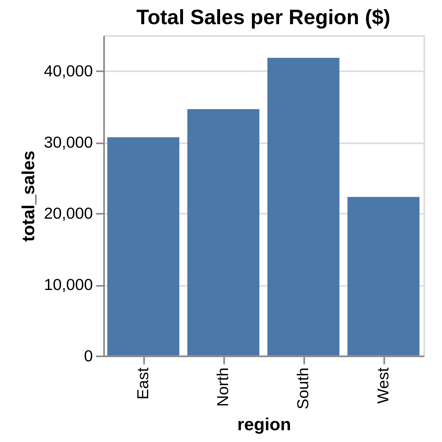
Remember, your figures will be different because their values are randomly generated.
Next, you’ll use pandas to produce a plot using the same data. Add a new cell to your Notebook, and add in the following code:
plots.ipynb
import pandas as pd

orders_pandas = pd.DataFrame(sales_data)

(
    orders_pandas.groupby(["region",])["sales_income"]
    .sum()
    .plot(kind="bar", title="Total Sales per Region ($)", ylabel="total_sales")
)
As before, you set up the same labels and titles. The pandas version of your plot looks like this:
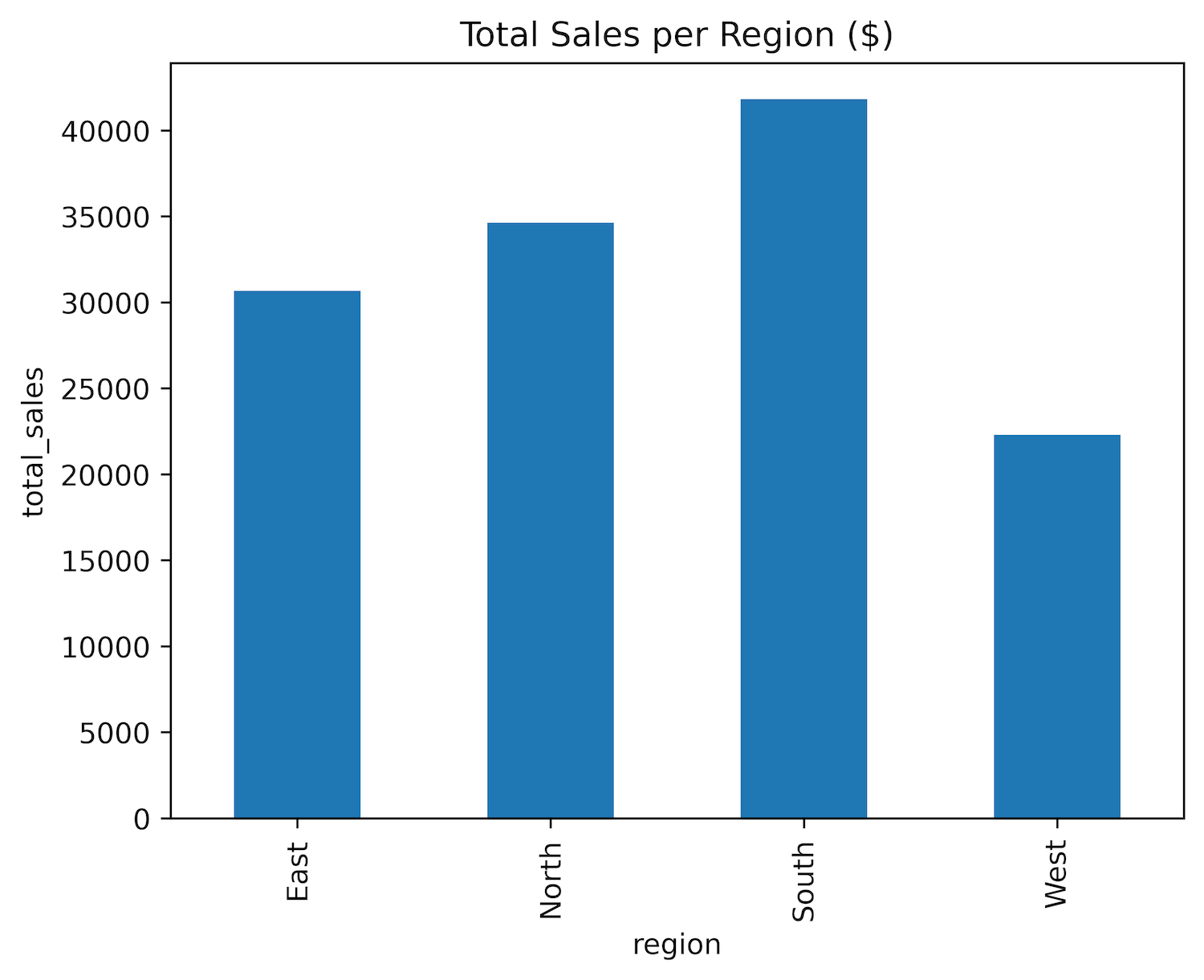
This plot should be similar to the previous version, but your plot will again differ from this one because of the random data used to construct them. It also looks slightly different from the previous one because you’re using a different library to produce it.
As you can see, you can quickly generate plots from within both pandas and Polars. It’s usually better to learn how to use the full features of these plotting libraries directly and feed your DataFrame columns into them. You need to use this technique if you choose to use the other plotting libraries that Python provides.
Are There Any Other Differences?
The pandas code is designed to be run on a computer’s CPU, and it does this very well. Polars also does this but can use your resources more efficiently. For example, it can use the cuDF library to delegate some of its processing to your computer’s GPU.
It’s possible to utilize parallelization in both pandas and Polars. This allows your computer to allocate different parts of the query across the other CPU cores in your system. However, to do this using pandas, you need to use a library such as Dask or Modin since pandas is single-threaded by default. Parallelization is built into Polars.
A vectorized query engine enables queries to be executed on groups of rows simultaneously, rather than processing them row by row. Both Polars and pandas support this. Currently, pandas relies on NumPy for vectorization, but starting with version 3 it will switch to PyArrow’s vectorization capabilities. Polars, by contrast, has a built-in SIMD (Single Instruction, Multiple Data) engine.
Although pandas is still the most popular of the two libraries because it’s been around for a lot longer and is more established, Polars is catching up. However, both are designed for single-node environments. If you need a solution that works in a distributed environment, then consider investigating a library such as PySpark.
Conclusion
By completing this tutorial, you’ve learned about the key differences between pandas and Polars, along with techniques to help you decide which one best fits your needs.
In this tutorial, you’ve learned that:
- Polars expressions and contexts let you build clear, optimized query pipelines without mutating your original data.
- LazyFrames with query optimization in Polars can outperform pandas for grouped and aggregated workloads.
- Streaming in Polars enables processing datasets that don’t fit in memory, which pandas can’t handle natively.
.to_pandas()andfrom_pandas()let you convert between DataFrame formats, and Narwhals offers a library-agnostic API.- Built-in plotting uses Altair for Polars and Matplotlib for pandas, allowing quick visualization directly from DataFrames.
You now understand the differences between the pandas and Polars libraries. To dive deeper, why not follow the links in this tutorial to explore the related topics in more detail?
Get Your Code: Click here to download the free sample code you’ll use to learn the differences between Polars and pandas.
Frequently Asked Questions
Now that you have some experience with Polars vs pandas in Python, you can use the questions and answers below to check your understanding and recap what you’ve learned.
These FAQs are related to the most important concepts you’ve covered in this tutorial. Click the Show/Hide toggle beside each question to reveal the answer.
You often see Polars run analysis faster than pandas, especially when you use LazyFrames and query optimization. For quick one-off tasks, you may find pandas faster to create the DataFrame, but Polars usually wins on grouped and aggregated workloads.
Yes, you may find Polars easier because it encourages clear method chaining with expressions and contexts. If you already think in NumPy-style indexing, you might prefer pandas, but chaining in Polars tends to read more cleanly for beginners.
Yes, you can chain pandas operations with methods like .assign(), .filter(), and .query() to build readable pipelines. You create new DataFrames at each step, so you avoid mutating your original data.
You call the DataFrame method .to_pandas() to get a pandas DataFrame. For the reverse process, you use Polars from_pandas(), and for mixed backends, you can wrap your data with Narwhals.
Yes, you can use Polars LazyFrames with streaming to process data in chunks without loading everything into RAM. pandas doesn’t offer built-in streaming, so you rely on Polars for this scenario.
Take the Quiz: Test your knowledge with our interactive “Polars vs pandas: What's the Difference?” quiz. You’ll receive a score upon completion to help you track your learning progress:
Interactive Quiz
Polars vs pandas: What's the Difference?Take this quiz to test your knowledge of the Polars vs pandas tutorial and review the key differences between these open-source Python libraries.