Have you ever wanted to compose music without expensive gear or a professional studio? Maybe you’ve tried to play a musical instrument before but found the manual dexterity required too daunting or time-consuming. If so, you might be interested in harnessing the power of Python to create a guitar synthesizer. By following a few relatively simple steps, you’ll be able to turn your computer into a virtual guitar that can play any song.
In this tutorial, you’ll:
- Implement the Karplus-Strong plucked string synthesis algorithm
- Mimic different types of string instruments and their tunings
- Combine multiple vibrating strings into polyphonic chords
- Simulate realistic guitar picking and strumming finger techniques
- Use impulse responses of real instruments to replicate their unique timbre
- Read musical notes from scientific pitch notation and guitar tablature
At any point, you’re welcome to download the complete source code of the guitar synthesizer, as well as the sample tablature and other resources that you’ll use throughout this tutorial. They might prove useful in case you want to explore the code in more detail or get a head start. To download the bonus materials now, visit the following link:
Get Your Code: Click here to download the free sample code that you’ll use to build a guitar synthesizer in Python.
Take the Quiz: Test your knowledge with our interactive “Build a Guitar Synthesizer” quiz. You’ll receive a score upon completion to help you track your learning progress:

Interactive Quiz
Build a Guitar SynthesizerIn this quiz, you'll test your understanding of what it takes to build a guitar synthesizer in Python. By working through this quiz, you'll revisit a few key concepts from music theory and sound synthesis.
Demo: Guitar Synthesizer in Python
In this step-by-step guide, you’ll build a plucked string instrument synthesizer based on the Karplus-Strong algorithm in Python. Along the way, you’ll create an ensemble of virtual instruments, including an acoustic, bass, and electric guitar, as well as a banjo and ukulele. Then, you’ll implement a custom guitar tab reader so that you can play your favorite songs.
By the end of this tutorial, you’ll be able to synthesize music from guitar tablature, or guitar tabs for short, which is a simplified form of musical notation that allows you to play music without having to learn how to read standard sheet music. Finally, you’ll store the result in an MP3 file for playback.
Below is a short demonstration of the synthesizer, re-creating the iconic soundtracks of classic video games like Doom and Diablo. Click the play button to listen to the sample output:
Once you find a guitar tab that you like, you can plug it into your Python guitar synthesizer and bring the music to life. For example, the Songsterr website is a fantastic resource with a wide range of songs you can choose from.
Project Overview
For your convenience, the project that you’re about to build, along with its third-party dependencies, will be managed by Poetry. The project will contain two Python packages with distinctly different areas of responsibility:
digitar: For the synthesis of the digital guitar soundtablature: For reading and interpreting guitar tablature from a file
You’ll also design and implement a custom data format to store guitar tabs on disk or in memory. This will allow you to play music based on a fairly standard tablature notation, which you’ll find in various places on the Internet. Your project will also provide a Python script to tie everything together, which will let you interpret the tabs with a single command right from your terminal.
Now, you can dive into the details of what you’ll need to set up your development environment and start coding.
Prerequisites
Although you don’t need to be a musician to follow along with this tutorial, a basic understanding of musical concepts such as notes, semitones, octaves, and chords will help you grasp the information more quickly. It’d also be nice if you had a rough idea of how computers represent and process digital audio in terms of sampling rate, bit depth, and file formats like WAV.
But don’t worry if you’re new to these ideas! You’ll be guided through each step in small increments with clear explanations and examples. So, even if you’ve never done any music synthesis before, you’ll have a working digital guitar or digitar by the end of this tutorial.
Note: You can learn music theory in half an hour by watching an excellent and free video by Andrew Huang.
The project that you’ll build was tested against Python 3.12 but should work fine in earlier Python versions, too, down to Python 3.10. In case you need a quick refresher, here’s a list of helpful resources covering the most important language features that you’ll take advantage of in your digital guitar journey:
- Assignment expressions
- Data classes
- Enumerations
- Protocols (static duck typing)
- Structural pattern matching
- Type hints
Other than that, you’ll use the following third-party Python packages in your project:
- NumPy to simplify and speed up the underlying sound synthesis
- Pedalboard to apply special effects akin to electric guitar amplifiers
- Pydantic and PyYAML to parse musical tablature representing finger movements on a guitar neck
Familiarity with these will definitely help, but you can also learn as you go and treat this project as an opportunity to practice and improve your Python skills.
Step 1: Set Up the Digital Guitar Project
The first step is to prepare your development environment. To start, you’ll create a new Python project and install the required third-party libraries. Then, you’ll load it into an editor, where you’ll continue to write the necessary code for your guitar synthesizer.
Create a New Project and Install Dependencies
There are many ways to create and manage Python projects. In this tutorial, you’ll use Poetry as a convenient tool for dependency management. If you haven’t already, then install Poetry—for example, with pipx—and start a new project using the src/ folder layout to keep your code organized:
$ poetry new --src --name digitar digital-guitar/
Created package digitar in digital-guitar
This will result in the folder structure below, which includes placeholder files with your project’s metadata and source code that you’ll fill out later:
digital-guitar/
│
├── src/
│   └── digitar/
│       └── __init__.py
│
├── tests/
│   └── __init__.py
│
├── pyproject.toml
└── README.md
Then, change the directory to your new project and add a few dependencies that you’ll rely on later:
$ cd digital-guitar/
$ poetry add numpy pedalboard pydantic pyyaml
After you run this command, Poetry will create an isolated virtual environment in a designated location for your project and install the listed third-party Python packages into it. You should also see a new poetry.lock file in your project’s root folder.
You can now open the digital-guitar/ folder in the Python IDE or code editor of your choice. If you use Visual Studio Code or PyCharm, then both programs will discover the virtual environment created by Poetry. The latter will also associate it with the project, letting you access the installed packages right away.
In VS Code, you may need to manually select the Poetry-managed virtual environment. To do this, bring up the Command Palette, type Python: Select Interpreter, and choose the desired interpreter. Conversely, after you open the folder in PyCharm, confirm the prompt asking you to set up a Poetry environment. The corresponding Python interpreter will appear in the bottom-right corner of the window.
Alternatively, if you’re a die-hard Vim or Sublime Text user, then you can continue to use Poetry in the command line:
$ poetry install
$ poetry run play-tab demo/tabs/doom.yaml
Saved file /home/user/digital-guitar/doom.mp3
The first command will install your project, along with its dependencies, defined in the pyproject.toml file. The second command, which you’ll implement later, will execute a script from within the associated virtual environment managed by Poetry. Note that you’ll use these commands anyway, regardless of which code editor you choose.
Embrace Immutable Data Types in Your Project
With only a few exceptions, you’ll define immutable data types almost exclusively in this project. Immutable objects are those that you can’t alter once you create them. While that may sound limiting at first, it actually brings a host of advantages. Therefore, it’s a good idea to familiarize yourself with the concept of immutability and its impact on your program’s behavior before you get started.
First of all, most immutable objects in Python are hashable, making them valid dictionary keys. Later, this will become essential for caching argument values to avoid repetitive computation. In the long run, it’ll help you reduce the overall time needed for sound synthesis.
Other than that, you can safely use immutable objects as default argument values without worrying about unintended side effects. In contrast, mutable default arguments are one of the most common pitfalls in Python, which can lead to surprising and difficult-to-track bugs. By sticking to immutable types where possible, you’ll save yourself a lot of headaches.
Also, you can think of immutable objects as simple values like integers or strings. When you assign an immutable variable to another variable, the assignment binds both references to the same object in memory. But, as soon as you attempt to modify the state of your immutable object through one of these variables, you’ll create a copy of that object, leaving the original one intact. Thus, your code becomes more predictable and resilient.
Immutable objects are also thread-safe and make it easier to reason about your code. These traits make them especially suitable for the functional programming paradigm, but you’ll enjoy their benefits in the object-oriented realm, too.
Now, it’s time to put this theory into practice by implementing your first immutable data type for this guitar synthesizer project.
Represent Time Instants, Durations, and Intervals
Music is an ephemeral form of art that you can only appreciate for a short period of time when it’s being played or performed. Because music inherently exists in time, it’s crucial that you’re able to properly represent time instants, durations, and intervals if you want to build a robust synthesizer.
Python’s float data type isn’t precise enough for musical timing due to the representation and rounding errors ingrained in the IEEE 754 standard. When you need greater precision, the recommended practice in Python is to replace floating-point numbers with either a Decimal or Fraction data type. However, using these types directly can be cumbersome, and they don’t carry the necessary information about the time units involved.
To alleviate these nuisances, you’ll implement a few custom classes, starting with the versatile Time data type. Go ahead and create a new Python module named temporal inside your digitar package, and define the following data class in it:
src/digitar/temporal.py
from dataclasses import dataclass
from decimal import Decimal
from fractions import Fraction
from typing import Self

type Numeric = int | float | Decimal | Fraction

@dataclass(frozen=True)
class Time:
    seconds: Decimal

    @classmethod
    def from_milliseconds(cls, milliseconds: Numeric) -> Self:
        return cls(Decimal(str(float(milliseconds))) / 1000)
This class has only one attribute, representing the number of seconds as a Decimal object for improved accuracy. You can create instances of your new class by providing the seconds through its constructor or by calling a class method that expects milliseconds and converts them to seconds wrapped in an appropriate data type.
Note: Since Python 3.12, you should use the type statement to create an explicit type alias. In previous Python releases, you can fall back to the deprecated TypeAlias annotation:
from typing import TypeAlias

Numeric: TypeAlias = int | float | Decimal | Fraction
Alternatively, if you’re running an even earlier version of Python, then just use a plain assignment statement without any keywords or annotations.
Due to Python’s dynamic nature, the default constructor generated by the interpreter for your data class won’t enforce type hints that you annotated your attributes with. In other words, the interpreter won’t verify whether the supplied values are of the expected types. So, in this case, if you pass an integer or a floating-point number instead of a Decimal object, then you’ll inadvertently create an instance with an incorrect attribute type.
Fortunately, you can prevent this issue by implementing your own initializer method in the class that will replace the one that Python generates by default:
src/digitar/temporal.py
from dataclasses import dataclass
from decimal import Decimal
from fractions import Fraction
from typing import Self

type Numeric = int | float | Decimal | Fraction

@dataclass(frozen=True)
class Time:
    seconds: Decimal

    @classmethod
    def from_milliseconds(cls, milliseconds: Numeric) -> Self:
        return cls(Decimal(str(float(milliseconds))) / 1000)

    def __init__(self, seconds: Numeric) -> None:
        match seconds:
            case int() | float():
                object.__setattr__(self, "seconds", Decimal(str(seconds)))
            case Decimal():
                object.__setattr__(self, "seconds", seconds)
            case Fraction():
                object.__setattr__(
                    self, "seconds", Decimal(str(float(seconds)))
                )
            case _:
                raise TypeError(
                    f"unsupported type '{type(seconds).__name__}'"
                )
You use structural pattern matching to detect the type of argument passed to your method at runtime and branch off accordingly. Then, you ensure that the instance attribute, .seconds, is always set to a Decimal object, regardless of the input type. If you pass a Decimal instance to your constructor, then there’s nothing more to do. Otherwise, you use the appropriate conversion or raise an exception to signal the misuse of the constructor.
Because you defined a frozen data class, which makes its instances immutable, you can’t set the attribute value directly or call the built-in setattr() function on an existing object. That would violate the immutability contract. If you ever need to forcefully change the state of a frozen data class instance, then you can resort to a hack by explicitly calling object.__setattr__(), as in the code snippet above.
You might recall that data classes support a special method for precisely this kind of customization. However, the advantage of overwriting the default initializer method instead of implementing .__post_init__() is that you take complete control of the object creation process. As a result, an object can either exist and be in a valid state or not exist at all.
Note: When creating an invalid object is essentially impossible, you can say that your code conforms to the fail-fast philosophy.
Finally, you can implement a convenience method that you’ll use later for translating a duration in seconds into the corresponding number of audio samples:
src/digitar/temporal.py
from dataclasses import dataclass
from decimal import Decimal
from fractions import Fraction
from typing import Self

type Numeric = int | float | Decimal | Fraction
type Hertz = int | float

@dataclass(frozen=True)
class Time:
    # ...

    def get_num_samples(self, sampling_rate: Hertz) -> int:
        return round(self.seconds * round(sampling_rate))
This method takes a sampling rate in hertz (Hz) as an argument, which represents the number of samples per second. Multiplying the duration in seconds by the sampling rate in hertz yields the required number of samples, which you can round to return an integer.
Here’s a short Python REPL session demonstrating how you can take advantage of your new data class:
>>> from digitar.temporal import Time

>>> Time(seconds=0.15)
Time(seconds=Decimal('0.15'))

>>> Time.from_milliseconds(2)
Time(seconds=Decimal('0.002'))

>>> _.get_num_samples(sampling_rate=44100)
88
The underscore (_) in the REPL is an implicit variable that holds the value of the last evaluated expression. In this case, it refers to your Time instance representing two milliseconds.
With the Time class in place, you’re ready to move on to the next step. You’ll dip your toes into the physics of a vibrating string and see how it produces a sound.
Step 2: Model the Acoustic Wave of a Vibrating String
At the end of the day, every sound that you hear is a local disturbance of air pressure made by a vibrating object. Whether it’s your vocal cords, a guitar string, or a loudspeaker, these vibrations push and pull on the air molecules around them. That movement then travels through the air as an acoustic wave until it reaches your eardrum, which vibrates in response.
In this step, you’ll take a closer look at the Karplus-Strong synthesis algorithm, which models the vibration of a plucked string. Then, you’ll implement it in Python using NumPy and produce your first synthetic sound resembling that of a plucked string.
Get to Know the Karplus-Strong Algorithm
The Karplus-Strong algorithm is surprisingly straightforward, given the complex sounds it can produce. In a nutshell, it starts by filling a very short buffer with a burst of random noise or another signal that has rich energy or many frequency components. That noise corresponds to the excitation of an actual string, which initially vibrates in several incoherent patterns of motion.
These seemingly random vibrations gradually become more and more sinusoidal, with a clear sine-like period and frequency that you perceive as a distinctive pitch. While the amplitudes of all vibrations weaken over time due to energy dissipation caused by internal friction and energy transfer, a certain fundamental frequency remains stronger than most of the overtones and harmonics that fade away more quickly.
Note: The string’s physical properties, including its length and mass, favor certain modes of vibration over others. That’s what inherently determines the particular frequency that persists and resonates most prominently.
In a guitar, you can shorten a string by pressing it against one of the frets on the guitar neck to produce a higher-pitched sound. Conversely, some strings are thicker and heavier than others, vibrating slower and resulting in lower-frequency sounds.
Additionally, the guitar’s bridge and nut are the anchor points that reflect the energy traveling back and forth along the string. These reflections interfere with waves that travel in opposite directions, contributing to the formation of standing waves, which are the basis of the musical notes that you hear.
Check out a slow-motion recording of a plucked string to see this phenomenon in action.
The Karplus-Strong algorithm applies a low-pass filter to the signal to simulate the decay of higher frequencies at a faster pace than the fundamental frequency. It does so by calculating a moving average of two consecutive amplitude levels in the buffer, effectively acting as a bare-bones convolution filter. It removes the short-term fluctuations while leaving the longer-term trend.
Additionally, the algorithm feeds the averaged values back into the buffer to reinforce and continue the vibration, albeit with gradual energy loss. Take a look at the diagram below to have a better picture of how this positive feedback loop works:
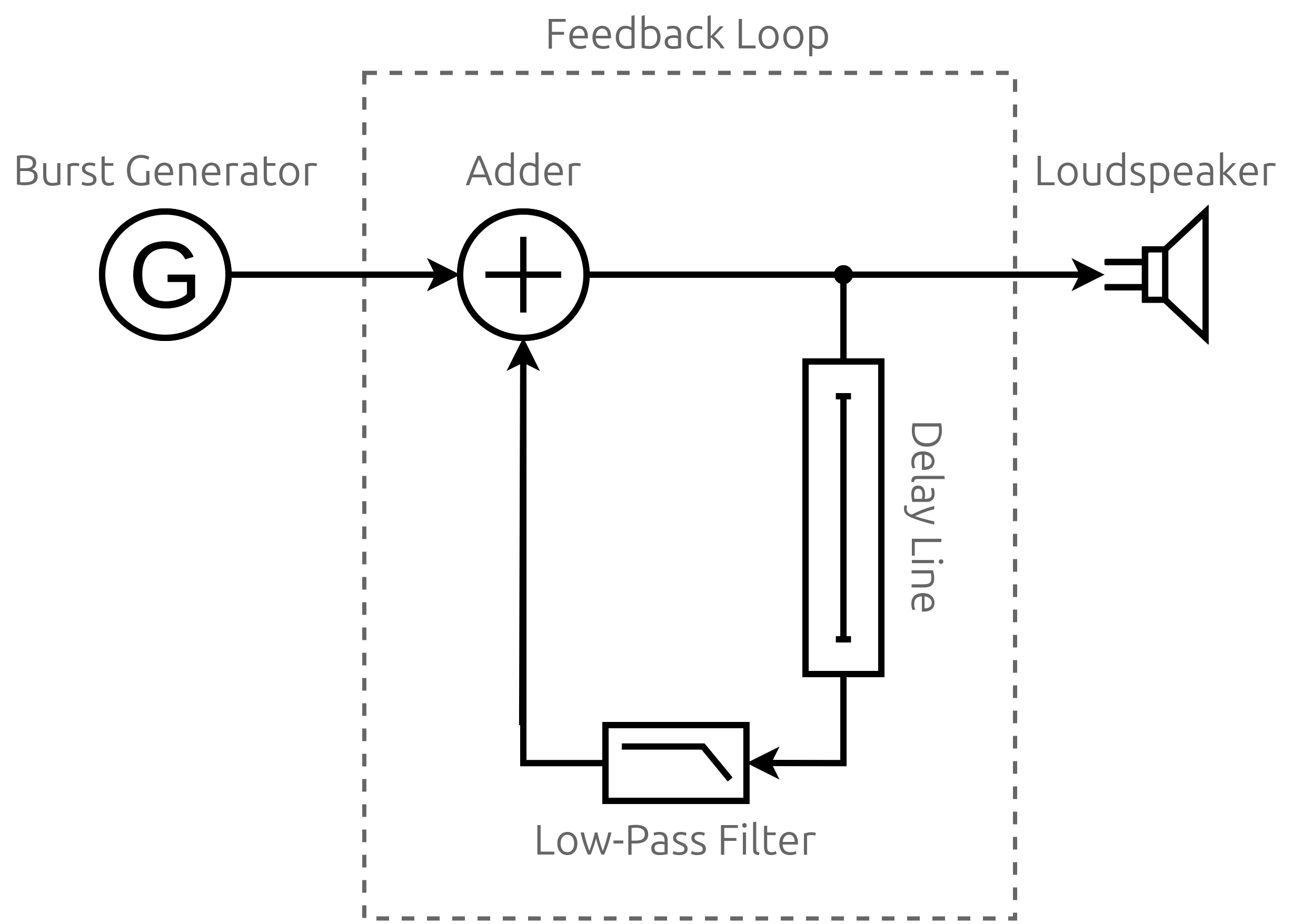
The generator on the left serves as the input to the algorithm, providing the initial burst of noise. It’ll typically be white noise with a uniform probability distribution so that, on average, no particular frequency is emphasized over another. The analogy is similar to white light, which contains all frequencies of the visible spectrum at roughly equal intensities.
The generator shuts down after filling a circular buffer, also known as the delay line, which delays the signal by a certain amount of time before feeding it back to the loop. The phase-shifted signal from the past is then mixed with the current signal. Think of it as the wave’s reflection propagating along the string in the opposite direction.
The amount of delay determines the frequency of the virtual string’s vibration. Just like with the guitar’s string length, a shorter delay results in a higher pitch, while a longer delay produces a lower pitch. You can calculate the required size of the buffer—in terms of the number of audio samples—using the following formula:

To get the number of samples, D, multiply the vibration’s period or the reciprocal of the desired fundamental frequency, F0, by your signal’s sampling frequency, Fs. Simply put, divide the sampling frequency by the fundamental frequency.
Then, the delayed signal goes through a low-pass filter before being added to the next sample from the buffer. You can implement both the filter and the adder by applying a weighted average to both samples as long as their weights sum to one or less. Otherwise, you’d be boosting the signal instead of attenuating it. By adjusting the weights, you can control the decay or damping of your virtual string’s vibration.
As the processed signal cycles through the buffer, it loses more high-frequency content and settles into a pattern that closely resembles the sound of a plucked string. Thanks to the feedback loop, you get the illusion of a vibrating string that gradually fades out.
Finally, on the far right of the diagram, you can see the output, which could be a loudspeaker or an audio file that you write the resulting audio samples to.
When you plot the waveforms and their corresponding frequency spectra from successive cycles of the feedback loop, you’ll observe the following pattern emerge:
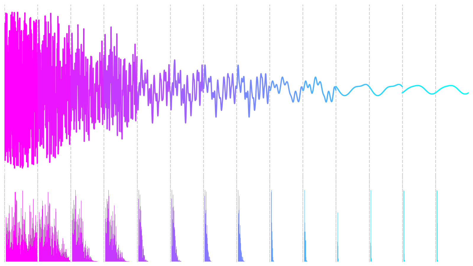
The top graph shows amplitude oscillations over time. The graph just below it depicts the signal’s frequency content at specific moments. Initially, the buffer is filled with random samples, whose frequency distribution is roughly equal across the spectrum. As time goes by, the signal’s amplitude decreases, and the frequency of oscillations starts to concentrate at a particular spectral band. The shape of the waveform resembles a sine wave now.
Since you now understand the principles of the Karplus-Strong algorithm, you can implement the first element of the diagram shown earlier.
Use Random Values as the Initial Noise Burst
There are many kinds of signal generators that you can choose from in sound synthesis. Some of the most popular ones include periodic functions like the square wave, triangle wave, and sawtooth wave. However, in the Karplus-Strong synthesis algorithm, you’ll get the best results with an aperiodic function, such as random noise, due to its rich harmonic content that you can filter over time.
Noise comes in different colors, like pink or white. The difference lies in their spectral power density across frequencies. In white noise, for example, each frequency band has approximately the same power. So, it’s perfect for an initial noise burst because it contains a wide range of harmonics that you can shape through a filter.
To allow for experimenting with the different kinds of signal generators, you’ll define a custom protocol class in a new Python module named burst:
src/digitar/burst.py
from typing import Protocol
import numpy as np
from digitar.temporal import Hertz

class BurstGenerator(Protocol):
    def __call__(self, num_samples: int, sampling_rate: Hertz) -> np.ndarray:
        ...
The point of a protocol class is to specify the desired behavior through method signatures without implementing those methods. In Python, you typically use an ellipsis (...) to indicate that you’ve intentionally left the method body undefined. Therefore, a protocol class acts like an interface in Java, where concrete classes implementing that particular interface provide the underlying logic.
Note: In Python, you’ll need a static type checker like mypy to enforce the protocol adherence by concrete classes.
In this case, you declared the special method .__call__()to make instances of classes that adhere to the protocol callable. Your method expects two arguments:
- The number of audio samples to produce
- The number of samples per second
Additionally, burst generators are meant to return a NumPy array of amplitude levels, which should be floating-point numbers normalized to an interval between minus one and plus one. Such normalization will make the subsequent audio processing more convenient.
Your first concrete generator class will produce white noise, as you’ve already established that it’s most appropriate in this context:
src/digitar/burst.py
# ...

class WhiteNoise:
    def __call__(self, num_samples: int, sampling_rate: Hertz) -> np.ndarray:
        return np.random.uniform(-1.0, 1.0, num_samples)
Even though your new class doesn’t inherit from BurstGenerator, it still conforms to the protocol you defined earlier by providing a .__call__() method with the correct signature. Notice that the method takes the sampling rate as the second argument despite not referencing it anywhere in the body. That’s required to satisfy the protocol.
Note: You’ll need to know the sampling rate for other types of burst generators, such as the periodic functions mentioned at the beginning of this section, which you might want to implement in the future.
Instances of your WhiteNoise generator class are callable now:
>>> from digitar.burst import WhiteNoise

>>> burst_generator = WhiteNoise()
>>> samples = burst_generator(num_samples=1_000_000, sampling_rate=44100)

>>> samples.min()
-0.9999988055552775

>>> samples.max()
0.999999948864092

>>> samples.mean()
-0.0001278112173601203
The resulting samples are constrained to the range between -1 and 1, as the minimum and maximum values are very close to these bounds. Also, the mean value is near zero because, over a large number of samples, the positive and negative amplitudes balance each other out, confirming a uniform value distribution.
Okay. The next big component in the diagram of the Karplus-Strong algorithm is the feedback loop itself. You’re going to break it down into smaller pieces now.
Filter Higher Frequencies With a Feedback Loop
An elegant way to simulate a feedback loop in Python entails wiring generator functions together and sending values to them. You can also define asynchronous functions and hook them up as cooperative coroutines to achieve a similar effect. However, in this tutorial, you’ll use a much more straightforward and slightly more efficient implementation based on iteration.
Create another module named synthesis in your Python package and define the following class placeholder:
src/digitar/synthesis.py
from dataclasses import dataclass
from digitar.burst import BurstGenerator, WhiteNoise

AUDIO_CD_SAMPLING_RATE = 44100

@dataclass(frozen=True)
class Synthesizer:
    burst_generator: BurstGenerator = WhiteNoise()
    sampling_rate: int = AUDIO_CD_SAMPLING_RATE
This frozen data class consists of two optional attributes, which let you specify the expected burst generator implementation and the sampling rate. If you skip those parameters when creating a new instance of the class, then you’ll rely on the defaults, which use the white noise generator at a 44.1 kHz sampling rate defined as a Python constant.
Note: The 44.1 kHz sampling rate is a common choice for audio applications like audio CDs. It means there are 44,100 samples of audio data recorded every second. That corresponds to a Nyquist frequency just above frequencies audible to the human ear, ensuring the accurate reproduction without aliasing artifacts.
Using the standard-library itertools package, you can now implement an infinite iterator that will cycle() through the buffer of audio samples. The following code snippet mirrors the Karplus-Strong diagram that you saw in an earlier section:
src/digitar/synthesis.py
from dataclasses import dataclass
from itertools import cycle
from typing import Iterator

import numpy as np

from digitar.burst import BurstGenerator, WhiteNoise
from digitar.temporal import Hertz, Time

AUDIO_CD_SAMPLING_RATE = 44100

@dataclass(frozen=True)
class Synthesizer:
    burst_generator: BurstGenerator = WhiteNoise()
    sampling_rate: int = AUDIO_CD_SAMPLING_RATE

    def vibrate(
        self, frequency: Hertz, duration: Time, damping: float = 0.5
    ) -> np.ndarray:
        assert 0 < damping <= 0.5

        def feedback_loop() -> Iterator[float]:
            buffer = self.burst_generator(
                num_samples=round(self.sampling_rate / frequency),
                sampling_rate=self.sampling_rate
            )
            for i in cycle(range(buffer.size)):
                yield (current_sample := buffer[i])
                next_sample = buffer[(i + 1) % buffer.size]
                buffer[i] = (current_sample + next_sample) * damping
You define the .vibrate() method that takes the vibration’s fundamental frequency, duration, and an optional damping coefficient as arguments. When left unspecified, the coefficient’s default value halves the sum of two adjacent samples with each cycle, which is analogous to computing a moving average. It simulates energy loss as the vibration fades out.
Note: To prevent passing in an incorrect damping coefficient, which would cause the algorithm to amplify the samples instead of damping them, you placed an assert statement with an appropriate condition at the beginning of your method. It’ll reject values outside the expected range, although you should only rely on such assertions during development. There are better ways to enforce invariants in your code that you’ll use later.
So far, your method defines an inner function that returns a generator iterator when called. The resulting generator object allocates and fills a buffer using the provided burst generator. The function then enters an infinite for loop that keeps yielding values from the buffer indefinitely in a round-robin fashion because it has no stopping condition.
You use the Walrus operator (:=) to simultaneously yield and intercept the current amplitude value in each cycle. On the next iteration, you calculate the average of the two adjacent values to simulate the damping effect. The modulo operator (%) ensures that the index wraps around to the beginning of the buffer once it reaches the end, creating a circular buffer effect.
To consume a finite number of samples determined by the duration parameter, you can wrap your feedback_loop() with a call to NumPy’s fromiter() function:
src/digitar/synthesis.py
# ...

@dataclass(frozen=True)
class Synthesizer:
    # ...

    def vibrate(
        self, frequency: Hertz, duration: Time, damping: float = 0.5
    ) -> np.ndarray:
        assert 0 < damping <= 0.5

        def feedback_loop() -> Iterator[float]:
            buffer = self.burst_generator(
                num_samples=round(self.sampling_rate / frequency),
                sampling_rate=self.sampling_rate
            )
            for i in cycle(range(buffer.size)):
                yield (current_sample := buffer[i])
                next_sample = buffer[(i + 1) % buffer.size]
                buffer[i] = (current_sample + next_sample) * damping

        return np.fromiter(
            feedback_loop(),
            np.float64,
            duration.get_num_samples(self.sampling_rate),
        )
As long as the duration parameter is an instance of the Time data class that you defined earlier, you can convert the number of seconds into the corresponding number of audio samples by calling .get_num_samples(). Just remember to pass the correct sampling rate. You should also specify float64 as the data type for the elements of your NumPy array to ensure high precision and avoid unnecessary type conversions.
Note: You want to take advantage of a high-precision numeric type during audio processing. However, you’ll usually encode the resulting audio samples with a more memory-efficient type, such as a 16-bit signed integer.
You’re almost done implementing the Karplus-Strong synthesis algorithm, but your code has two minor issues that you need to address first.
Remove the DC Bias and Normalize Audio Samples
Depending on the initial burst and the damping coefficient, you may end up with values outside the expected amplitude range, or the values may drift away from zero, introducing a DC bias. That could result in audible clicks or other unpleasant artifacts. To fix these potential problems, you’ll remove the bias by subtracting the signal’s mean value, and you’ll normalize the resulting samples afterward.
NumPy doesn’t provide built-in functions for these tasks, but making your own isn’t too complicated. Start by creating a new module named processing in your package with these two functions:
src/digitar/processing.py
import numpy as np

def remove_dc(samples: np.ndarray) -> np.ndarray:
    return samples - samples.mean()

def normalize(samples: np.ndarray) -> np.ndarray:
    return samples / np.abs(samples).max()
Both functions take advantage of NumPy’s vectorization capabilities. The first one subtracts the mean value from each element, and the second divides all samples by the maximum absolute value in the input array.
Now, you can import and call your helper functions in the synthesizer before returning the array of computed audio samples:
src/digitar/synthesis.py
from dataclasses import dataclass
from itertools import cycle
from typing import Iterator

import numpy as np

from digitar.burst import BurstGenerator, WhiteNoise
from digitar.processing import normalize, remove_dc
from digitar.temporal import Hertz, Time

AUDIO_CD_SAMPLING_RATE = 44100

@dataclass(frozen=True)
class Synthesizer:
    # ...

    def vibrate(
        self, frequency: Hertz, duration: Time, damping: float = 0.5
    ) -> np.ndarray:
        # ...
        return normalize(
            remove_dc(
                np.fromiter(
                    feedback_loop(),
                    np.float64,
                    duration.get_num_samples(self.sampling_rate),
                )
            )
        )
Although the order may not make a significant difference, it’s customary to remove the DC bias before performing the normalization. Removing the DC component ensures that your signal is centered around zero. Otherwise, it might still have a DC component, which could affect the overall scale of the normalization.
Great! You’ve just implemented the Karplus-Strong synthesis algorithm in Python. Why not put it to the test to hear the results?
Pluck the String to Produce Monophonic Sounds
Strictly speaking, your synthesizer returns a NumPy array of normalized amplitude levels instead of audio samples directly corresponding to digital sound. At the same time, you can choose from several data formats, compression schemes, and encodings to determine how to store and transmit your audio data.
For example, Linear Pulse-Code Modulation (LPCM) is a standard encoding in uncompressed WAV files, which typically use 16-bit signed integers to represent audio samples. Other formats like MP3 employ lossy compression algorithms that reduce file size by removing information that’s less perceivable by the human ear. These formats can offer constant or variable bitrates depending on the desired quality and file size.
To avoid getting bogged down by the technicalities, you’ll use Spotify’s Pedalboard library, which can handle these low-level details for you. You’ll supply the normalized amplitude levels from your synthesizer, and Pedalboard will encode them accordingly depending on your preferred data format:
>>> from pedalboard.io import AudioFile

>>> from digitar.synthesis import Synthesizer
>>> from digitar.temporal import Time

>>> frequencies = [261.63, 293.66, 329.63, 349.23, 392, 440, 493.88, 523.25]
>>> duration = Time(seconds=0.5)
>>> damping = 0.495

>>> synthesizer = Synthesizer()
>>> with AudioFile("monophonic.mp3", "w", synthesizer.sampling_rate) as file:
...     for frequency in frequencies:
...         file.write(synthesizer.vibrate(frequency, duration, damping))
In this case, you save the synthesized sounds as an MP3 file using the library’s default parameters. The code snippet above produces an MP3 file with a mono channel sampled at 44.1 kHz and a constant bitrate of 320 kilobits per second, which is the highest quality supported by this format. Remember to run the code from within your project’s virtual environment to access the required modules.
To confirm some of these audio properties, you can open the file for reading and check a few of its attributes:
>>> with AudioFile("monophonic.mp3") as file:
...     print(f"{file.num_channels = }")
...     print(f"{file.samplerate = }")
...     print(f"{file.file_dtype = }")
...
file.num_channels = 1
file.samplerate = 44100
file.file_dtype = 'float32'
Because MP3 files are compressed, you can’t calculate their bitrate from these parameters. The actual bitrate is stored in the file’s header along with other metadata, which you can verify using an external program like MediaInfo:
$ mediainfo monophonic.mp3
General
Complete name                            : monophonic.mp3
Format                                   : MPEG Audio
File size                                : 159 KiB
Duration                                 : 4 s 48 ms
Overall bit rate mode                    : Constant
Overall bit rate                         : 320 kb/s
Writing library                          : LAME3.100
(...)
The generated file contains a series of musical tones based on the frequencies that you supplied. Each tone is sustained for half a second, resulting in a melody that progresses through the notes do-re-mi-fa-sol-la-ti-do. These tones are the solfeggio notes, often used to teach the musical scale. Below is what they look like when plotted as a waveform. You can click the play button to take a listen:
Notice that each tone stops abruptly before getting a chance to fade out completely. You can experiment with a longer or shorter duration and adjust the the damping parameter. But, no matter how hard you try, you can only produce monophonic sounds without the possibility of overlaying multiple notes.
In the next section, you’ll learn how to synthesize more complex sounds, getting one step closer to simulating a full-fledged guitar.
Step 3: Simulate Strumming Multiple Guitar Strings
At this point, you can generate audio files consisting of monophonic sounds. This means that as soon as the next sound starts playing, the previous one stops, resulting in a series of discrete tones. That’s fine for old-school cellphone ringtones or retro video game soundtracks. However, when a guitarist strums several strings at once, they produce a chord with notes that resonate together.
In this section, you’ll tweak your synthesizer class to produce polyphonic sounds by allowing the individual notes to overlap and interfere with each other.
Blend Multiple Notes Into a Polyphonic Sound
To play multiple notes simultaneously, you can mix the corresponding acoustic waves. Go ahead and define another method in your synthesizer class, which will be responsible for overlaying samples from multiple sounds on top of each other:
src/digitar/synthesis.py
from dataclasses import dataclass
from itertools import cycle
from typing import Iterator, Sequence

# ...

@dataclass(frozen=True)
class Synthesizer:
    # ...

    def overlay(self, sounds: Sequence[np.ndarray]) -> np.ndarray:
        return np.sum(sounds, axis=0)
This method takes a sequence of equal-sized NumPy arrays comprising the amplitudes of several sounds to mix. The method then returns the element-wise arithmetic sum of the input sound waves.
Note: While you should generally remain flexible by allowing your functions and methods to take any iterable as their input arguments, in this case, NumPy expects the iterable to have a fixed size.
Assuming you’ve already removed the DC bias from the individual sounds you want to mix, you no longer need to worry about it. Additionally, you don’t want to normalize the overlaid sounds at this stage because their number may vary greatly within a single song. Doing so now could lead to inconsistent volume levels, making certain musical chords barely audible. Instead, you must apply normalization before writing the entire song into the file.
Suppose you wanted to simulate a performer plucking all the strings of a guitar at the same time. Here’s how you could do that using your new method:
>>> from pedalboard.io import AudioFile

>>> from digitar.processing import normalize
>>> from digitar.synthesis import Synthesizer
>>> from digitar.temporal import Time

>>> frequencies = [329.63, 246.94, 196.00, 146.83, 110.00, 82.41]
>>> duration = Time(seconds=3.5)
>>> damping = 0.499

>>> synthesizer = Synthesizer()
>>> sounds = [
...     synthesizer.vibrate(frequency, duration, damping)
...     for frequency in frequencies
... ]

>>> with AudioFile("polyphonic.mp3", "w", synthesizer.sampling_rate) as file:
...     file.write(normalize(synthesizer.overlay(sounds)))
You define the frequencies corresponding to the standard tuning of a six-string guitar and set the duration of an individual note to three and a half seconds. Additionally, you adjust the damping coefficient to a slightly greater value than before to make it vibrate longer. Then, you synthesize each string’s sound in a list comprehension and combine them using your .overlay() method.
This will be the resulting waveform of the audio file that you’ll create after you run the code listed above:
It’s unquestionably an improvement over the monophonic version. However, the synthesized file still sounds a bit artificial when you play it. That’s because, with a real guitar, the strings are never plucked at precisely the same moment. There’s always a slight delay between each string being plucked. The resulting wave interactions create complex resonances, adding to the richness and authenticity of the sound.
Next, you’ll introduce an adjustable delay between the subsequent strokes to give your polyphonic sound a more realistic feel. You’ll be able to discern the striking direction as a result of that!
Adjust the Stroke Speed to Control the Rhythm
When you stroke the strings of a guitar quickly, the delay between successive plucks is relatively short, making the overall sound loud and sharp. Conversely, the delay increases as you pluck the strings more slowly and gently. You can take this technique to the extreme by playing an arpeggio or a broken chord where you play the notes one after the other rather than simultaneously.
Now, modify your .overlay() method so that it accepts an additional delay parameter representing the time interval between each stroke:
src/digitar/synthesis.py
# ...

@dataclass(frozen=True)
class Synthesizer:
    # ...

    def overlay(
        self, sounds: Sequence[np.ndarray], delay: Time
    ) -> np.ndarray:
        num_delay_samples = delay.get_num_samples(self.sampling_rate)
        num_samples = max(
            i * num_delay_samples + sound.size
            for i, sound in enumerate(sounds)
        )
        samples = np.zeros(num_samples, dtype=np.float64)
        for i, sound in enumerate(sounds):
            offset = i * num_delay_samples
            samples[offset : offset + sound.size] += sound
        return samples
Based on the current sampling frequency of your synthesizer, you convert the delay in seconds into the corresponding number of samples. Then, you find the total number of samples to allocate for the resulting array, which you initialize with zeros. Finally, you iterate over the sounds, adding them into your samples array with the appropriate offset.
Note: This modified version of .overlay() lets you mix variable-length sounds whose arrays no longer have to be of equal size. That can be particularly handy if you want to allow one or more strings to ring out longer than the rest, creating an interesting texture.
Here’s the same example you saw in the previous section. However, you now have a forty-millisecond delay between the individual plucks, and you vary the vibration duration depending on its frequency:
>>> from pedalboard.io import AudioFile

>>> from digitar.processing import normalize
>>> from digitar.synthesis import Synthesizer
>>> from digitar.temporal import Time

>>> frequencies = [329.63, 246.94, 196.00, 146.83, 110.00, 82.41]
>>> delay = Time.from_milliseconds(40)
>>> damping = 0.499

>>> synthesizer = Synthesizer()
>>> sounds = [
...     synthesizer.vibrate(frequency, Time(3.5 + 0.25 * i), damping)
...     for i, frequency in enumerate(frequencies)
... ]

>>> with AudioFile("arpeggio.mp3", "w", synthesizer.sampling_rate) as file:
...     file.write(normalize(synthesizer.overlay(sounds, delay)))
Notes with a lower frequency will have a slightly longer duration than their higher-frequency counterparts. This simulates the inertia of real strings, which tend to vibrate longer if they are thicker or longer.
Below is the corresponding waveform, which appears to have more variation and complexity:
If you look closely at this waveform, then you’ll see the individual peaks at the beginning, indicating where the subsequent notes start. They’re equally spaced, as determined by your delay parameter.
By changing the delay, you can adjust the stroke speed to create a faster and more dynamic rhythm or a slower, more mellow sound. You’ll use this parameter to enhance the expressiveness of your virtual instrument and mimic the musical phrasings that a guitarist might naturally use.
Now that you have control over the timing of each note in a chord, you can experiment further by changing the order in which you play them.
Reverse the Strumming Direction to Alter the Timbre
Guitarists often vary not just the speed but also the strumming direction as they play. By alternating between downstrokes and upstrokes, they can emphasize different strings and change the timbre of the same chord. Downstrokes tend to sound more powerful and are usually louder because the pick—or your finger—hits the lower, thicker strings first. Conversely, upstrokes often highlight the higher, thinner strings, producing a lighter sound.
You can express both the strumming speed and direction with custom data types. Create a Python module named stroke in your digitar package and define these two classes in it:
src/digitar/stroke.py
import enum
from dataclasses import dataclass
from typing import Self

from digitar.temporal import Time

class Direction(enum.Enum):
    DOWN = enum.auto()
    UP = enum.auto()

@dataclass(frozen=True)
class Velocity:
    direction: Direction
    delay: Time

    @classmethod
    def down(cls, delay: Time) -> Self:
        return cls(Direction.DOWN, delay)

    @classmethod
    def up(cls, delay: Time) -> Self:
        return cls(Direction.UP, delay)
The first class is a Python enumeration, which assigns unique values to the mutually exclusive stroke directions, of which there are two. The following class, Velocity, uses that enumeration as its member, combining it with the delay or the interval between the subsequent plucks.
You can quickly instantiate objects to represent guitar strokes by calling convenient class methods on your Velocity class:
>>> from digitar.stroke import Direction, Velocity
>>> from digitar.temporal import Time

>>> slow = Time.from_milliseconds(40)
>>> fast = Time.from_milliseconds(20)

>>> Velocity.down(slow)
Velocity(direction=<Direction.DOWN: 1>, delay=Time(seconds=Decimal('0.04')))

>>> Velocity.up(fast)
Velocity(direction=<Direction.UP: 2>, delay=Time(seconds=Decimal('0.02')))
The first stroke is slow and directed downward, while the second is faster and directed upward. You’ll use these new data types in the project to control the musical feel of your digital guitar.
But there are many kinds of guitars in the wild. Some have fewer strings, others are bigger or smaller, and some need an electronic amplifier. On top of that, you can tune each instrument to different notes. So, before you can properly take advantage of the stroke velocity, you need to build a virtual instrument and learn how to handle it.
Step 4: Play Musical Notes on the Virtual Guitar
At this point, you can produce monophonic as well as polyphonic sounds based on specific frequencies with your digital guitar. In this step, you’ll model the relationship between those frequencies and the musical notes they correspond to. Additionally, you’ll simulate the tuning of the guitar strings and the interaction with the fretboard to create a realistic playing experience.
Press a Vibrating String to Change Its Pitch
Most guitars have between four and twelve strings, each capable of producing a variety of pitches. When you pluck an open string without touching the guitar neck, the string starts to vibrate at its fundamental frequency. However, once you press the string against one of the metal strips or frets along the fingerboard, you effectively shorten the string, changing its vibration frequency when plucked.
Note: The shorter the string, the higher the frequency of vibration or pitch that you can hear. Conversely, the longer the string, the lower the pitch. That’s why a double bass has such a long neck, and a ukulele has a shorter one.
Each guitar fret represents an increase in pitch by a single semitone or a half-step on the chromatic scale—the standard scale in Western music. The chromatic scale divides each octave, or a set of eight musical notes, into twelve equally spaced semitones, with a ratio of the twelfth root of two between them. When you go all the way up to the twelfth semitone, you’ll double the frequency of the note that marks the beginning of an octave.
The distances between adjacent frets in a fretted instrument follow the same principle, reflecting the logarithmic nature of the frequency increase at each step. As you move along the fretboard and press down on successive frets, you’ll notice the pitch of the string progressively increasing, one semitone at a time.
On a typical six-string guitar, you’ll usually find about twenty or more frets, amounting to over a hundred pitches! However, when you account for the duplicates due to overlapping octaves, the actual number of distinctive pitches decreases. In reality, you can play about four octaves of musical notes, which is short of fifty unique pitches. On the other hand, the virtual guitar that you’re about to build has no such limits!
In Python, you can implement a semitone-based pitch adjustment like this:
src/digitar/pitch.py
from dataclasses import dataclass
from typing import Self

from digitar.temporal import Hertz

@dataclass(frozen=True)
class Pitch:
    frequency: Hertz

    def adjust(self, num_semitones: int) -> Self:
        return Pitch(self.frequency * 2 ** (num_semitones / 12))
Once you create a new pitch, you can modify the corresponding fundamental frequency by calling .adjust() with the desired number of semitones. A positive number of semitones will increase the frequency, a negative number will decrease it, while zero will keep it intact. Note that you use Python’s exponentiation operator (**) to calculate the twelfth root of two, which the formula relies on.
To confirm that your code is working as expected, you can run the following test:
>>> from digitar.pitch import Pitch

>>> pitch = Pitch(frequency=110.0)
>>> semitones = [-12, 12, 24] + list(range(12))

>>> for num_semitones in sorted(semitones):
...     print(f"{num_semitones:>3}: {pitch.adjust(num_semitones)}")
...
-12: Pitch(frequency=55.0)
  0: Pitch(frequency=110.0)
  1: Pitch(frequency=116.54094037952248)
  2: Pitch(frequency=123.47082531403103)
  3: Pitch(frequency=130.8127826502993)
  4: Pitch(frequency=138.59131548843604)
  5: Pitch(frequency=146.8323839587038)
  6: Pitch(frequency=155.56349186104046)
  7: Pitch(frequency=164.81377845643496)
  8: Pitch(frequency=174.61411571650194)
  9: Pitch(frequency=184.9972113558172)
 10: Pitch(frequency=195.99771799087463)
 11: Pitch(frequency=207.65234878997256)
 12: Pitch(frequency=220.0)
 24: Pitch(frequency=440.0)
You start by defining a pitch produced by a string vibrating at 110 Hz, which corresponds to the A note in the second octave. Then, you iterate over a list of semitone numbers to adjust the pitch accordingly.
Depending on whether the given number is negative or positive, adjusting the frequency by exactly twelve semitones (one octave) either halves or doubles the original frequency of that pitch. Anything in between sets the frequency to the corresponding semitone within that octave.
Note: In all cases, you get a new instance of the Pitch class, which is immutable.
Being able to adjust the frequency is useful, but the Pitch class forces you to think in terms of pitches, semitones, and octaves, which isn’t the most convenient. You’ll wrap the pitch in a higher-level class inside a new module named instrument:
src/digitar/instrument.py
from dataclasses import dataclass

from digitar.pitch import Pitch

@dataclass(frozen=True)
class VibratingString:
    pitch: Pitch

    def press_fret(self, fret_number: int | None = None) -> Pitch:
        if fret_number is None:
            return self.pitch
        return self.pitch.adjust(fret_number)
To simulate plucking an open string, pass None or leave the fret_number parameter out when calling your .press_fret() method. By doing so, you’ll return the string’s unaltered pitch. Alternatively, you can pass zero as the fret number.
And here’s how you can interact with your new class:
>>> from digitar.instrument import VibratingString
>>> from digitar.pitch import Pitch

>>> a2_string = VibratingString(Pitch(frequency=110))

>>> a2_string.pitch
Pitch(frequency=110)

>>> a2_string.press_fret(None)
Pitch(frequency=110)

>>> a2_string.press_fret(0)
Pitch(frequency=110.0)

>>> a2_string.press_fret(1)
Pitch(frequency=116.54094037952248)

>>> a2_string.press_fret(12)
Pitch(frequency=220.0)
You can now treat pitches and guitar strings independently, which lets you assign a different pitch to the same string if you want to. This mapping of pitches to open strings is known as guitar tuning in music. Tuning systems require you to understand a specific notation of musical notes, which you’ll learn about in the next section.
Read Musical Notes From Scientific Pitch Notation
In scientific pitch notation, every musical note appears as a letter followed by an optional symbol, such as a sharp (♯) or flat (♭) denoting accidentals, as well as an octave number. The sharp symbol raises the note’s pitch by a semitone, while the flat symbol lowers it by a semitone. If you omit the octave number, then zero is assumed implicitly.
There are seven letters in this notation, with C marking the boundaries of each octave:
| Semitone | 1 | 2 | 3 | 4 | 5 | 6 | 7 | 8 | 9 | 10 | 11 | 12 | 13 |
|---|---|---|---|---|---|---|---|---|---|---|---|---|---|
| Sharp | C♯0 | D♯0 | F♯0 | G♯0 | A♯0 | ||||||||
| Tone | C0 | D0 | E0 | F0 | G0 | A0 | B0 | C1 | |||||
| Flat | D♭0 | E♭0 | G♭0 | A♭0 | B♭0 |
In this case, you’re looking at the first octave comprising eight notes: C0, D0, E0, F0, G0, A0, B0, and C1. The system starts at C0 or just C, which is approximately 16.3516 Hz. When you go all the way up to C1 on the right, which also starts the next octave, you’ll double that frequency.
Note: While most letters are a whole tone apart, not all of them have sharp or flat equivalents. The letters E and F, as well as B and C, are already one half-tone apart, so there’s no E♯ or F♭. This is for historical reasons due to the technical limitations of the early piano keyboards:
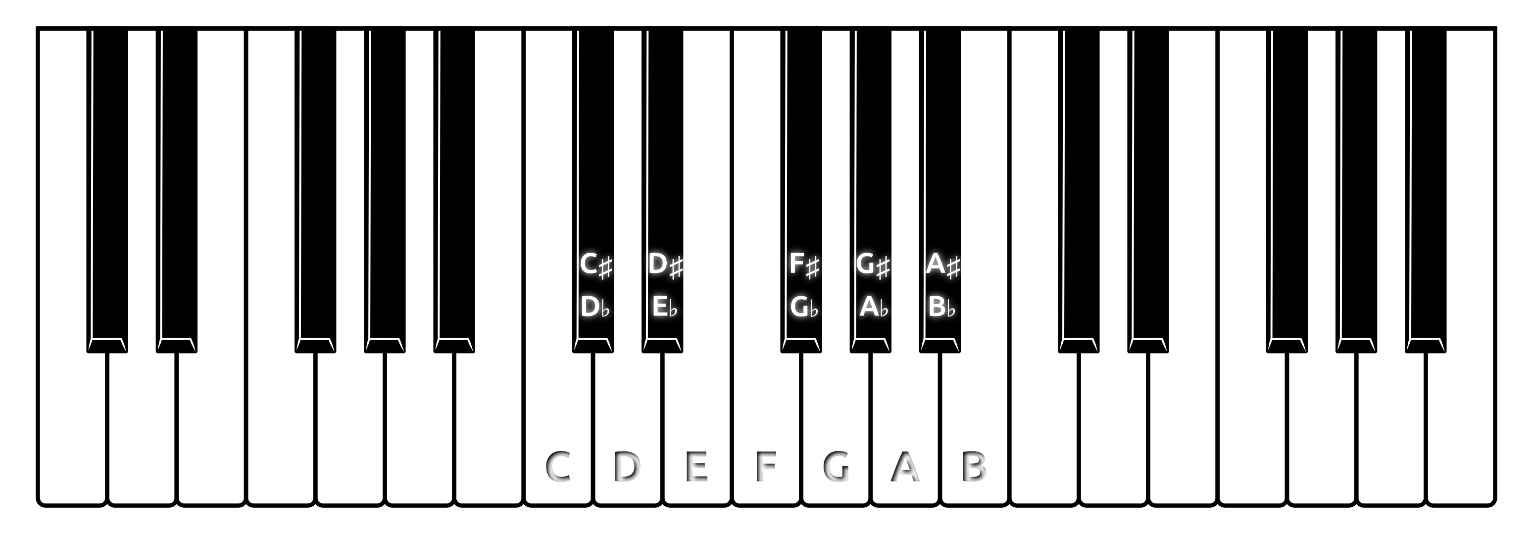
When you overlay the notes in scientific pitch notation on top of a piano keyboard, you’ll notice that accidentals correspond to the five black keys. Conversely, the natural tones correspond to the seven white keys in each octave that repeat in both directions across the keyboard.
You can now decipher scientific pitch notation. For example, A4 indicates the musical note A in the fourth octave, with a frequency of 440 Hz, which is the concert pitch reference. Similarly, C♯4 represents the C-sharp note in the fourth octave, located one semitone above the middle C on a standard piano keyboard.
In Python, you can leverage regular expressions to programmatically translate this notation into numeric pitches. Add the following class method to the Pitch class in the pitch module:
src/digitar/pitch.py
import re
from dataclasses import dataclass
from typing import Self

from digitar.temporal import Hertz

@dataclass(frozen=True)
class Pitch:
    frequency: Hertz

    @classmethod
    def from_scientific_notation(cls, notation: str) -> Self:
        if match := re.fullmatch(r"([A-G]#?)(-?\d+)?", notation):
            note = match.group(1)
            octave = int(match.group(2) or 0)
            semitones = "C C# D D# E F F# G G# A A# B".split()
            index = octave * 12 + semitones.index(note) - 57
            return cls(frequency=440.0 * 2 ** (index / 12))
        else:
            raise ValueError(
                f"Invalid scientific pitch notation: {notation}"
            )

    def adjust(self, num_semitones: int) -> Self:
        return Pitch(self.frequency * 2 ** (num_semitones / 12))
This method calculates the frequency for a given note based on its distance in semitones from A4. Note that this is a simplified implementation, which only takes sharp notes into account. If you need to represent a flat note, then you can rewrite it in terms of its equivalent sharp note, provided that it exists. For instance, B♭ is the same as A♯.
Here’s the sample usage of your new class method:
>>> from digitar.pitch import Pitch
>>> for note in "C", "C0", "A#", "C#4", "A4":
...     print(f"{note:>3}", Pitch.from_scientific_notation(note))
...
  C Pitch(frequency=16.351597831287414)
 C0 Pitch(frequency=16.351597831287414)
 A# Pitch(frequency=29.13523509488062)
C#4 Pitch(frequency=277.1826309768721)
 A4 Pitch(frequency=440.0)
As you can see, the code accepts and interprets a few variants of scientific pitch notation. That’s perfect! You’re now ready to tune up your digital guitar.
Perform String Tuning of the Virtual Guitar
In the real world, musicians adjust the tension of guitar strings by tightening or loosening the respective tuning pegs to achieve a perfectly tuned sound. Doing so allows them to assign different sets of musical notes or pitches to their instrument’s strings. They’ll occasionally reuse the same pitch for two or more strings to create a fuller sound.
Depending on the number of strings in a guitar, you’ll assign the musical notes differently. Apart from the standard tuning, which is the most typical choice of notes for a given instrument, you can apply several alternative guitar tunings, even when you have the same number of strings at your disposal.
The traditional six-string guitar tuning, from the thinnest string (highest pitch) to thickest one (lowest pitch), is the following:
| String | Note | Frequency |
|---|---|---|
| 1st | E4 | 329.63 Hz |
| 2nd | B3 | 246.94 Hz |
| 3rd | G3 | 196.00 Hz |
| 4th | D3 | 146.83 Hz |
| 5th | A2 | 110.00 Hz |
| 6th | E2 | 82.41 Hz |
If you’re right-handed, you’d typically use your right hand to strum or pluck the strings near the sound hole while your left hand frets the notes on the neck. In this orientation, the first string (E4) is closest to the bottom, while the sixth string (E2) is closest to the top.
It’s customary to denote guitar tunings in ascending frequency order. For example, the standard guitar tuning is usually presented as: E2-A2-D3-G3-B3-E4. At the same time, some guitar tabs follow the string numbering depicted in the table above, which reverses this order. Therefore, the top line in a six-string guitar tablature will usually represent the first string (E4) and the bottom line the sixth string (E2).
To avoid confusion, you’ll respect both conventions. Add the following class to your instrument module so that you can represent a string tuning:
src/digitar/instrument.py
from dataclasses import dataclass
from typing import Self

from digitar.pitch import Pitch

# ...

@dataclass(frozen=True)
class StringTuning:
    strings: tuple[VibratingString, ...]

    @classmethod
    def from_notes(cls, *notes: str) -> Self:
        return cls(
            tuple(
                VibratingString(Pitch.from_scientific_notation(note))
                for note in reversed(notes)
            )
        )
An object of this class contains a tuple of VibratingString instances sorted by the string number in ascending order. In other words, the first element in the tuple corresponds to the first string (E4) and the last element to the sixth string (E2). Note that the number of strings can be less than or greater than six should you need to represent other types of stringed instruments, such as a banjo, which has just five strings.
In practice, you’ll create new instances of the StringTuning class by calling the .from_notes() class method and passing a variable number of musical notes in scientific pitch notation. When you do, you must follow the string tuning order, starting with the lowest pitch. This is because the method reverses the input notes to match the typical string arrangement on a guitar tab.
Here’s how you might use the StringTuning class to represent various tuning systems for different plucked string instruments:
>>> from digitar.instrument import StringTuning

>>> StringTuning.from_notes("E2", "A2", "D3", "G3", "B3", "E4")
StringTuning(
    strings=(
        VibratingString(pitch=Pitch(frequency=329.6275569128699)),
        VibratingString(pitch=Pitch(frequency=246.94165062806206)),
        VibratingString(pitch=Pitch(frequency=195.99771799087463)),
        VibratingString(pitch=Pitch(frequency=146.8323839587038)),
        VibratingString(pitch=Pitch(frequency=110.0)),
        VibratingString(pitch=Pitch(frequency=82.4068892282175)),
    )
)

>>> StringTuning.from_notes("E1", "A1", "D2", "G2")
StringTuning(
  strings=(
    VibratingString(pitch=Pitch(frequency=97.99885899543733)),
    VibratingString(pitch=Pitch(frequency=73.41619197935188)),
    VibratingString(pitch=Pitch(frequency=55.0)),
    VibratingString(pitch=Pitch(frequency=41.20344461410875)),
  )
)
The first object represents the standard six-string guitar tuning, while the second one represents the four-string bass guitar tuning. You can use the same approach to model the tuning of other stringed instruments by providing the appropriate notes for each string.
With this, you can achieve the effect of fretting the guitar with your fingers to play a particular chord:
>>> tuning = StringTuning.from_notes("E2", "A2", "D3", "G3", "B3", "E4")
>>> frets = (None, None, 2, None, 0, None)
>>> for string, fret_number in zip(tuning.strings, frets):
...     if fret_number is not None:
...         string.press_fret(fret_number)
...
Pitch(frequency=220.0)
Pitch(frequency=110.0)
In this case, you use the standard guitar tuning. Then, you simulate pressing the second fret on the third string (G3) and leaving the fifth string (A2) open while strumming both of them. You don’t stroke or fret the remaining strings, as indicated by None in the tuple. The zip() function combines strings and the corresponding fret numbers into pairs that you iterate over.
Note: The number of frets must correspond to the number of guitar strings. Otherwise, you risk indexing errors or inaccurate representation of the chord being played.
The third string is tuned to note G3 or 196 Hz. But, since you press it on the second fret, you increase its pitch by two semitones, resulting in a frequency of 220 Hz. The fifth string is tuned to A2 or 110 Hz, which you play open or without fretting. When you mix both frequencies, you’ll produce a chord consisting of notes A3 and A2, which are one octave apart.
Note: Such a combination of musical notes creates a unison or perfect octave interval, which is harmonically consonant and pleasing to the ear.
Next up, you’ll create a custom data type to represent musical chords more conveniently.
Represent Chords on a Fretted Instrument
Previously, you defined a plain tuple to express the fret numbers in a particular chord. You can be a tad bit more explicit by extending the tuple class and restricting the types of values that are allowed in it:
src/digitar/chord.py
from typing import Self

class Chord(tuple[int | None, ...]):
    @classmethod
    def from_numbers(cls, *numbers: int | None) -> Self:
        return cls(numbers)
With type hints, you declare that your tuple should only contain integers representing the fret numbers or empty values (None) indicating an open string. You also provide a class method, .from_numbers(), allowing you to create a Chord instance by passing in the fret numbers directly. This method takes a variable number of arguments, each of which can be an integer or None.
Note: Python tuples are immutable, so you don’t need to take extra steps to follow your initial design goals.
Here’s how you might define a chord from the previous section of this tutorial using the Chord class:
>>> from digitar.chord import Chord

>>> Chord.from_numbers(None, None, 2, None, 0, None)
(None, None, 2, None, 0, None)

>>> Chord([None, None, 2, None, 0, None])
(None, None, 2, None, 0, None)
When you create a Chord instance using the class method, you pass the fret numbers as arguments. You can also instantiate the class by passing an iterable object of values, such as a list, to the constructor. However, it’s generally more explicit to use the .from_numbers() method.
To sum up, these are the most important points to remember:
- The value’s position in the tuple determines the string number, so the first element corresponds to the highest pitch.
- An empty value (
None) means that you don’t pluck the string at all. - Zero represents an open string, which you pluck without pressing any frets.
- Other integers correspond to fret numbers on a guitar neck that you press.
These are also finger patterns on guitar tabs that you’ll leverage later in the tutorial. Now, it’s time to define another custom data type with which you’ll represent different kinds of plucked string instruments in code.
Model Any Plucked String Instrument
When you think about the primary properties that influence how a plucked string instrument sounds, they’re the number of strings, their tuning, and the material they’re made of. While not the only one, the latter aspect affects how long the string will sustain its vibration and the degree of energy damping.
You can conveniently express those attributes by defining a data class in your instrument module:
src/digitar/instrument.py
from dataclasses import dataclass
from typing import Self

from digitar.pitch import Pitch
from digitar.temporal import Time

# ...

@dataclass(frozen=True)
class PluckedStringInstrument:
    tuning: StringTuning
    vibration: Time
    damping: float = 0.5

    def __post_init__(self) -> None:
        if not (0 < self.damping <= 0.5):
            raise ValueError(
                "string damping must be in the range of (0, 0.5]"
            )
The string tuning determines how many strings an instrument has and what their fundamental frequencies of vibration are. For simplicity, all strings in an instrument will share the same vibration time and damping coefficient that defaults to one-half. If you’d like to override them individually on a string-by-string basis, then you’ll need to tweak the code yourself.
The .__post_init__() method verifies whether the damping is within the acceptable range of values.
You can define a convenient property in your class to quickly find out the number of strings in an instrument without reaching out for the tuning object:
src/digitar/instrument.py
from dataclasses import dataclass
from functools import cached_property
from typing import Self

from digitar.pitch import Pitch
from digitar.temporal import Time

# ...

@dataclass(frozen=True)
class PluckedStringInstrument:
    # ...

    @cached_property
    def num_strings(self) -> int:
        return len(self.tuning.strings)
It’s a cached property for more efficient access. After you access such a property for the first time, Python remembers the computed value, so subsequent accesses won’t recompute it since the value doesn’t change during an object’s lifetime.
Next, you may add methods that will take a Chord instance, which you built earlier, and turn it into a tuple of pitches that you can later use to synthesize a polyphonic sound:
src/digitar/instrument.py
from dataclasses import dataclass
from functools import cache, cached_property
from typing import Self

from digitar.chord import Chord
from digitar.pitch import Pitch
from digitar.temporal import Time

# ...

@dataclass(frozen=True)
class PluckedStringInstrument:
    # ...

    @cache
    def downstroke(self, chord: Chord) -> tuple[Pitch, ...]:
        return tuple(reversed(self.upstroke(chord)))

    @cache
    def upstroke(self, chord: Chord) -> tuple[Pitch, ...]:
        if len(chord) != self.num_strings:
            raise ValueError(
                "chord and instrument must have the same string count"
            )
        return tuple(
            string.press_fret(fret_number)
            for string, fret_number in zip(self.tuning.strings, chord)
            if fret_number is not None
        )
Since the order of fret numbers in a chord agrees with the order of guitar strings (bottom-up), stroking a chord simulates an upstroke. Your .upstroke() method uses a generator expression with a conditional expression, which looks almost identical to the loop you saw earlier when you performed the string tuning. The .downstroke() method delegates execution to .upstroke(), intercepts the resulting tuple of the Pitch objects, and reverses it.
Because most chords repeat over and over again in similar patterns within a single song, you don’t want to calculate each one of them every time. Instead, you annotate both methods with the @cache decorator to avoid redundant computations. By storing the computed tuples, Python will return the cached result when the same inputs occur again.
You can now model different types of plucked string instruments to reproduce their unique acoustic characteristics. Here are a few examples using the standard tuning of each instrument:
>>> from digitar.instrument import PluckedStringInstrument, StringTuning
>>> from digitar.temporal import Time

>>> acoustic_guitar = PluckedStringInstrument(
...     tuning=StringTuning.from_notes("E2", "A2", "D3", "G3", "B3", "E4"),
...     vibration=Time(seconds=10),
...     damping=0.498,
... )

>>> bass_guitar = PluckedStringInstrument(
...     tuning=StringTuning.from_notes("E1", "A1", "D2", "G2"),
...     vibration=Time(seconds=10),
...     damping=0.4965,
... )

>>> electric_guitar = PluckedStringInstrument(
...     tuning=StringTuning.from_notes("E2", "A2", "D3", "G3", "B3", "E4"),
...     vibration=Time(seconds=0.09),
...     damping=0.475,
... )

>>> banjo = PluckedStringInstrument(
...     tuning=StringTuning.from_notes("G4", "D3", "G3", "B3", "D4"),
...     vibration=Time(seconds=2.5),
...     damping=0.4965,
... )

>>> ukulele = PluckedStringInstrument(
...     tuning=StringTuning.from_notes("A4", "E4", "C4", "G4"),
...     vibration=Time(seconds=5.0),
...     damping=0.498,
... )
Right now, they’re only abstract containers for logically related data. Before you can take full advantage of these virtual instruments and actually hear them, you must integrate them into your Karplus-Strong synthesizer, which you’ll do next.
Combine the Synthesizer With an Instrument
You want to parameterize your synthesizer with a plucked string instrument so that you can synthesize sounds that are characteristic of that particular instrument. Open the synthesis module in your Python project now and add an instrument field to the Synthesizer class:
src/digitar/synthesis.py
from dataclasses import dataclass
from itertools import cycle
from typing import Sequence

import numpy as np

from digitar.burst import BurstGenerator, WhiteNoise
from digitar.instrument import PluckedStringInstrument
from digitar.processing import normalize, remove_dc
from digitar.temporal import Hertz, Time

AUDIO_CD_SAMPLING_RATE = 44100

@dataclass(frozen=True)
class Synthesizer:
    instrument: PluckedStringInstrument
    burst_generator: BurstGenerator = WhiteNoise()
    sampling_rate: int = AUDIO_CD_SAMPLING_RATE

    # ...
By using the properties defined in the PluckedStringInstrument class, the synthesizer can generate sounds that mimic the timbre and expression of a plucked string instrument, such as an acoustic guitar or a banjo.
Now that you have an instrument in your synthesizer, you can leverage its tuned strings to play a chord with the given speed and direction:
src/digitar/synthesis.py
# ...

from digitar.burst import BurstGenerator, WhiteNoise
from digitar.chord import Chord
from digitar.instrument import PluckedStringInstrument
from digitar.processing import normalize, remove_dc
from digitar.stroke import Direction, Velocity
from digitar.temporal import Hertz, Time

AUDIO_CD_SAMPLING_RATE = 44100

@dataclass(frozen=True)
class Synthesizer:
    instrument: PluckedStringInstrument
    burst_generator: BurstGenerator = WhiteNoise()
    sampling_rate: int = AUDIO_CD_SAMPLING_RATE

    def strum_strings(
        self, chord: Chord, velocity: Velocity, vibration: Time | None = None
    ) -> np.ndarray:
        if vibration is None:
            vibration = self.instrument.vibration

        if velocity.direction is Direction.UP:
            stroke = self.instrument.upstroke
        else:
            stroke = self.instrument.downstroke

        sounds = tuple(
            self.vibrate(pitch.frequency, vibration, self.instrument.damping)
            for pitch in stroke(chord)
        )

        return self.overlay(sounds, velocity.delay)

    # ...
Your new .strum_strings() method expects a Chord and a Velocity instance at the minimum. You can optionally pass the vibration duration, but if you don’t, then the method falls back on the instrument’s default duration. Depending on the desired stroke direction, it synthesizes the pitches in ascending or descending string order. Finally, it overlays them with the required delay or arpeggiation.
Note: You could introduce two separate methods, one for plucking an individual string and another one for strumming multiple strings at once. However, it’s more convenient to treat both cases uniformly, especially when you have to deal with hundreds of chords in a guitar tablature.
Because .strum_strings() has become the only part of the public interface of your class, you can signal that the other two methods, vibrate() and overlay(), are intended for internal use only. A common convention in Python to denote non-public methods is to prefix their names with a single underscore (_):
src/digitar/synthesis.py
# ...

@dataclass(frozen=True)
class Synthesizer:
    # ...

    def strum_strings(...) -> np.ndarray:
        # ...

        sounds = tuple(
            self._vibrate(pitch.frequency, vibration, self.instrument.damping)
            for pitch in stroke(chord)
        )

        return self._overlay(sounds, velocity.delay)

    def _vibrate(...) -> np.ndarray:
        # ...

    def _overlay(...) -> np.ndarray:
        # ...
It’s clear now that ._vibrate() and ._overlay() are implementation details that can change without notice, so you shouldn’t access them from an external scope.
Your synthesizer is almost complete, but it’s missing one crucial detail. If you were to synthesize a complete music piece, like the original Diablo soundtrack, then over ninety percent of the synthesis time would be spent on redundant computation. That’s because most songs consist of repeating patterns and motifs. It’s these repeated sequences of chords that create a recognizable rhythm.
To bring down the total synthesis time from minutes to seconds, you can incorporate caching of the intermediate results. Ideally, you’d want to decorate all methods in your Synthesizer class with the @cache decorator to compute them once for each unique list of arguments. However, caching requires that all method arguments are hashable.
While you diligently used immutable objects, which also happen to be hashable, NumPy arrays aren’t. Therefore, you can’t cache the results of your ._overlay() method, which takes a sequence of arrays as an argument. Instead, you can cache the other two methods that only rely on immutable objects:
src/digitar/synthesis.py
from dataclasses import dataclass
from functools import cache
from itertools import cycle
from typing import Sequence

# ...

@dataclass(frozen=True)
class Synthesizer:
    # ...

    @cache
    def strum_strings(...) -> np.ndarray:
        # ...

    @cache
    def _vibrate(...) -> np.ndarray:
        # ...

    def _overlay(...) -> np.ndarray:
        # ...
With this little change, you essentially trade storage for speed. As long as your computer has enough memory, it’ll only take a fraction of the time it would have otherwise. Since the results are stored and retrieved, they won’t be recalculated each time they’re requested.
Note: Caching works best with so-called pure functions, whose output can be completely determined by the input. If your function causes side effects or depends on a global state, then you’re better off without caching.
How about playing a few chords on some of your instruments? Below is a short code snippet that plays a downstroke strum on all open strings of three different plucked string instruments you defined earlier:
>>> from pedalboard.io import AudioFile

>>> from digitar.chord import Chord
>>> from digitar.instrument import PluckedStringInstrument, StringTuning
>>> from digitar.stroke import Direction, Velocity
>>> from digitar.synthesis import Synthesizer
>>> from digitar.temporal import Time

>>> instruments = {
...     "acoustic_guitar": PluckedStringInstrument(
...         tuning=StringTuning.from_notes("E2", "A2", "D3", "G3", "B3", "E4"),
...         vibration=Time(seconds=10),
...         damping=0.498,
...     ),
...     "banjo": PluckedStringInstrument(
...         tuning=StringTuning.from_notes("G4", "D3", "G3", "B3", "D4"),
...         vibration=Time(seconds=2.5),
...         damping=0.4965,
...     ),
...     "ukulele": PluckedStringInstrument(
...         tuning=StringTuning.from_notes("A4", "E4", "C4", "G4"),
...         vibration=Time(seconds=5.0),
...         damping=0.498,
...     ),
... }

>>> for name, instrument in instruments.items():
...     synthesizer = Synthesizer(instrument)
...     amplitudes = synthesizer.strum_strings(
...         Chord([0] * instrument.num_strings),
...         Velocity(Direction.DOWN, Time.from_milliseconds(40))
...     )
...     with AudioFile(f"{name}.mp3", "w", synthesizer.sampling_rate) as file:
...         file.write(amplitudes)
This code iterates through a dictionary of key-value pairs consisting of the instrument’s name and the corresponding PluckedStringInstrument instance. When you play the resulting audio files below, you’ll recognize the distinctive timbre of each instrument:
Alright. You have all the pieces together and are ready to play real music on your virtual guitar!
Step 5: Compose Melodies With Strumming Patterns
At this point, you can synthesize the individual notes and chords, which sound like you played them on an actual instrument. Additionally, you can simulate different types of plucked string instruments and tune them to your liking. In this part of the tutorial, you’ll compose more complex melodies from these building blocks.
Allocate an Audio Track for Your Instrument
Music is made up of chords and notes arranged along a linear timeline, intentionally spaced to create rhythm and melody. A single song often contains more than one audio track corresponding to different instruments, such as lead guitar, bass guitar, and drums, as well as vocals.
You’ll represent an audio track with your first mutable class in this project to allow for incrementally adding and mixing sounds in chronological order. Define a new module named track with the following AudioTrack class in it:
src/digitar/track.py
import numpy as np

from digitar.temporal import Hertz, Time

class AudioTrack:
    def __init__(self, sampling_rate: Hertz) -> None:
        self.sampling_rate = int(sampling_rate)
        self.samples = np.array([], dtype=np.float64)

    def __len__(self) -> int:
        return self.samples.size

    @property
    def duration(self) -> Time:
        return Time(seconds=len(self) / self.sampling_rate)

    def add(self, samples: np.ndarray) -> None:
        self.samples = np.append(self.samples, samples)
An audio track contains a sequence of audio samples, or more precisely, the amplitude levels that you’ll encode as samples with a chosen data format. However, you’ll refer to them as samples to keep things simple.
To make a new instance of your AudioTrack class, you need to provide the desired sampling rate or frequency in hertz. It’ll let you calculate the track’s current duration in seconds, as well as add new samples at a specific time offset. As of now, you can only append samples at the very end of your existing track without the possibility of overlaying them earlier or inserting them later.
You’ll fix that now by implementing another method in your class:
src/digitar/track.py
# ...

class AudioTrack:
    # ...

    def add_at(self, instant: Time, samples: np.ndarray) -> None:
        samples_offset = round(instant.seconds * self.sampling_rate)
        if samples_offset == len(self):
            self.add(samples)
        elif samples_offset > len(self):
            self.add(np.zeros(samples_offset - len(self)))
            self.add(samples)
        else:
            end = samples_offset + len(samples)
            if end > len(self):
                self.add(np.zeros(end - len(self)))
            self.samples[samples_offset:end] += samples
This method, .add_at(), takes a time instant as an argument in addition to the sequence of samples to add. Based on the track’s sampling rate, it calculates the offset in terms of the number of audio samples. If the offset aligns with the current length of the audio track, then the method appends the samples by means of delegation to the .add() method.
Otherwise, the logic gets slightly more involved:
- Gap: If the offset is beyond the current length of the track, then the method fills the gap with zeros before appending the new samples as before.
- Full Overlap: If the offset is somewhere in the middle of the track and the new samples can fit within it, then the method overlays the new samples on top of the existing ones at the correct position.
- Partial Overlap: If the offset is somewhere in the middle of the track but the new samples reach beyond its current end, then the method blends the overlapping part and appends the remaining samples that extend beyond the current track length.
The new method lets you precisely place sounds within an audio track. But you still need to keep track of the progression of time on the timeline. You’ll create another custom data type to help you with that.
Track the Music Progression on a Timeline
Time can only move forward, so you’ll model the timeline as another mutable class with a special method for advancing the current instant. Open your temporal module now and add the following data class definition:
src/digitar/temporal.py
# ...

@dataclass
class Timeline:
    instant: Time = Time(seconds=0)

    def __rshift__(self, seconds: Numeric | Time) -> Self:
        self.instant += seconds
        return self
Unless you specify otherwise, a timeline starts at zero seconds by default. Thanks to the immutability of Time objects, you can use one as a default value for the instant attribute.
The .__rshift__() method provides the implementation of the bitwise right shift operator (>>) for your class. In this case, it’s a non-standard implementation, which has nothing to do with operations on bits. Instead, it advances the timeline by a given number of seconds or another Time object. The method updates the current Timeline instance in place and returns itself, allowing for method chaining or evaluating the shifted timeline right away.
Notice that shifting the timeline adds either a numeric value, such as a Decimal object, or a Time instance to another Time instance. This addition won’t work out of the box because Python doesn’t know how to add two objects of custom data types using the plus operator (+). Fortunately, you can tell it how to handle such an addition by implementing the .__add__() method in your Time class:
src/digitar/temporal.py
# ...

@dataclass(frozen=True)
class Time:
    # ...

    def __add__(self, seconds: Numeric | Self) -> Self:
        match seconds:
            case Time() as time:
                return Time(self.seconds + time.seconds)
            case int() | Decimal():
                return Time(self.seconds + seconds)
            case float():
                return Time(self.seconds + Decimal(str(seconds)))
            case Fraction():
                return Time(Fraction.from_decimal(self.seconds) + seconds)
            case _:
                raise TypeError(f"can't add '{type(seconds).__name__}'")

    def get_num_samples(self, sampling_rate: Hertz) -> int:
        return round(self.seconds * round(sampling_rate))

# ...
When you provide a Time object as an argument to .__add__(), then the method calculates the sum of the decimal seconds in both instances and returns a new Time instance with the resulting seconds. On the other hand, if the argument is one of the expected numeric types, then the method converts it appropriately first. In case of an unsupported type, the method raises an exception with an error message.
Review the following examples to understand how you can use the Timeline class:
>>> from digitar.temporal import Time, Timeline

>>> Timeline()
Timeline(instant=Time(seconds=Decimal('0')))

>>> Timeline(instant=Time.from_milliseconds(100))
Timeline(instant=Time(seconds=Decimal('0.1')))

>>> Timeline() >> 0.1 >> 0.3 >> 0.5
Timeline(instant=Time(seconds=Decimal('0.9')))

>>> from digitar.temporal import Time, Timeline
>>> timeline = Timeline()
>>> for offset in 0.1, 0.3, 0.5:
...     timeline >> offset
...
Timeline(instant=Time(seconds=Decimal('0.1')))
Timeline(instant=Time(seconds=Decimal('0.4')))
Timeline(instant=Time(seconds=Decimal('0.9')))

>>> timeline.instant.seconds
Decimal('0.9')
These examples showcase various ways of using the overridden bitwise operator to move through time. In particular, you can chain multiple time increments in one expression to advance the timeline cumulatively. A timeline is persistent, so any previous changes are retained in it, letting you query the current instant.
With an audio track and a timeline, you can finally compose your first melody. Are you ready to have some fun?
Repeat Chords in Spaced Time Intervals
For starters, you’ll play the chorus from Jason Mraz’s hit song “I’m Yours” on a virtual ukulele. The following example is based on an excellent explanation generously provided by Adrian from the Learn And Play channel on YouTube. If you’re interested in learning more about how to play this particular song, then check out a much more involved video tutorial on Adrian’s sister channel.
Note: The mentioned video tutorial was recorded in Polish, which is Adrian’s mother tongue. Unfortunately, there are no English subtitles available for this video, so you might need to use third-party tools for automated transcription and translation to understand the lesson.
The chorus of the song consists of four chords in the following sequence with their corresponding fingering patterns for a ukulele:
- C major: Press the third fret on the first string
- G major: Press the second fret on the first string, the third fret on the second string, and the second fret on the third string
- A minor: Press the second fret on the fourth string
- F major: Press the first fret on the second string and the second fret on the fourth string
Additionally, each chord should be played according to the strumming pattern depicted below, repeated twice:
- Downstroke (slow)
- Downstroke (slow)
- Upstroke (slow)
- Upstroke (fast)
- Downstroke (fast)
- Upstroke (slow)
In other words, you begin by placing your fingers on the fretboard to form the desired chord, and then you keep stroking the strings in the prescribed pattern. When you reach the end of that pattern, you rinse and repeat by playing through it once more for the same chord. After you’ve strummed through the pattern twice for a particular chord, you move on to the next chord in the sequence.
The subsequent strokes in the pattern are spaced roughly at these time intervals in seconds:
| 0.65s | 0.45s | 0.75s | 0.2s | 0.4s | 0.25s |
While the specific chord offsets were estimated by ear, they’re good enough for the sake of this exercise. You’ll use them to spread the synthesized chords across an audio track with the help of a timeline.
Putting it together, you can create a Python script named play_chorus.py that replicates the strumming pattern of the song’s chorus. To keep things tidy, consider making a new subfolder in your project’s root folder, where you’ll store such scripts. For example, you can give it the name demo/:
demo/play_chorus.py
from itertools import cycle
from typing import Iterator

from digitar.chord import Chord
from digitar.stroke import Velocity
from digitar.temporal import Time

def strumming_pattern() -> Iterator[tuple[float, Chord, Velocity]]:
    chords = (
        Chord.from_numbers(0, 0, 0, 3),
        Chord.from_numbers(0, 2, 3, 2),
        Chord.from_numbers(2, 0, 0, 0),
        Chord.from_numbers(2, 0, 1, 0),
    )

    fast = Time.from_milliseconds(10)
    slow = Time.from_milliseconds(25)

    strokes = [
        Velocity.down(slow),
        Velocity.down(slow),
        Velocity.up(slow),
        Velocity.up(fast),
        Velocity.down(fast),
        Velocity.up(slow),
    ]

    interval = cycle([0.65, 0.45, 0.75, 0.2, 0.4, 0.25])

    for chord in chords:
        for _ in range(2):  # Repeat each chord twice
            for stroke in strokes:
                yield next(interval), chord, stroke
The strumming_pattern() function above returns an iterator of triplets, consisting of the time interval in seconds, a Chord instance, and a Velocity object that describes a stroke. The interval is an offset of the next chord on the timeline relative to the current chord.
Each chord indicates the fret numbers to press on the respective strings. Remember that strings are counted from the right side, so the last element in the chord’s tuple represents the first string.
There are four types of strokes in total. Both upstroke and downstroke come in two flavors: slow and fast, which differ in the amount of delay between the consecutive plucks. You alternate between these strokes to simulate the expected rhythm.
Next, you can define a virtual ukulele and hook it up to the synthesizer:
demo/play_chorus.py
from itertools import cycle
from typing import Iterator

from digitar.chord import Chord
from digitar.instrument import PluckedStringInstrument, StringTuning
from digitar.stroke import Velocity
from digitar.synthesis import Synthesizer
from digitar.temporal import Time

def main() -> None:
    ukulele = PluckedStringInstrument(
        tuning=StringTuning.from_notes("A4", "E4", "C4", "G4"),
        vibration=Time(seconds=5.0),
        damping=0.498,
    )
    synthesizer = Synthesizer(ukulele)

# ...

if __name__ == "__main__":
    main()
Following Python’s name-main idiom, you define the main() function as the entry point to your script, and you call it at the bottom of the file. Then, you reuse the PluckedStringInstrument definition that you saw in an earlier section, which specifies the standard tuning of a ukulele.
The next step is to synthesize the individual chords—depending on how you stroke your virtual strings—and add them to an audio track at the right moment:
demo/play_chorus.py
from itertools import cycle
from typing import Iterator

from digitar.chord import Chord
from digitar.instrument import PluckedStringInstrument, StringTuning
from digitar.stroke import Velocity
from digitar.synthesis import Synthesizer
from digitar.temporal import Time, Timeline
from digitar.track import AudioTrack

def main() -> None:
    ukulele = PluckedStringInstrument(
        tuning=StringTuning.from_notes("A4", "E4", "C4", "G4"),
        vibration=Time(seconds=5.0),
        damping=0.498,
    )
    synthesizer = Synthesizer(ukulele)
    audio_track = AudioTrack(synthesizer.sampling_rate)
    timeline = Timeline()
    for interval, chord, stroke in strumming_pattern():
        audio_samples = synthesizer.strum_strings(chord, stroke)
        audio_track.add_at(timeline.instant, audio_samples)
        timeline >> interval

# ...
Based on the synthesizer’s sampling rate, you create an audio track and a timeline that starts at zero seconds. You then iterate over the strumming pattern, synthesize the next ukulele sound, and add it to the audio track at the current instant. Lastly, you advance the timeline using the provided offset.
You can now save the amplitudes retained in your audio track to a file, remembering to normalize them to avoid clipping and other distortion:
demo/play_chorus.py
from itertools import cycle
from typing import Iterator

from pedalboard.io import AudioFile

from digitar.chord import Chord
from digitar.instrument import PluckedStringInstrument, StringTuning
from digitar.processing import normalize
from digitar.stroke import Velocity
from digitar.synthesis import Synthesizer
from digitar.temporal import Time, Timeline
from digitar.track import AudioTrack

def main() -> None:
    ukulele = PluckedStringInstrument(
        tuning=StringTuning.from_notes("A4", "E4", "C4", "G4"),
        vibration=Time(seconds=5.0),
        damping=0.498,
    )
    synthesizer = Synthesizer(ukulele)
    audio_track = AudioTrack(synthesizer.sampling_rate)
    timeline = Timeline()
    for interval, chord, stroke in strumming_pattern():
        audio_samples = synthesizer.strum_strings(chord, stroke)
        audio_track.add_at(timeline.instant, audio_samples)
        timeline >> interval

    with AudioFile("chorus.mp3", "w", audio_track.sampling_rate) as file:
        file.write(normalize(audio_track.samples))

# ...
When you run this script, you’ll end up with an audio file named chorus.mp3, which records the strumming pattern and chords of the song:
Give yourself a well-deserved pat on the back! You’ve just made a plucked string instrument synthesizer. It works decently well but requires you to manually schedule the individual notes on the timeline to match the rhythm. That can be error-prone and clunky. Plus, you can’t change the song’s tempo or the number of beats per minute.
Next up, you’ll take a more systematic approach to arranging the musical notes and chords on the timeline.
Divide the Timeline Into Measures of Beats
Music revolves around time, which is central to rhythm, tempo, and the duration of the individual notes within a composition. Throughout history, composers have found it convenient to divide the timeline into segments known as measures or bars, usually containing an equal number of beats.
You can think of the beat as the basic unit of time in a musical composition. It’s a steady pulse that determines the rhythm. The beat typically remains consistent throughout a song, and you can intuitively recognize it by tapping your feet or clapping your hands to it. Musicians sometimes deliberately count beats out loud or in their heads to maintain the timing of their performance.
Each measure has an associated time signature consisting of two numbers stacked vertically. The top number indicates how many beats are in the measure, and the bottom number denotes a fractional note value, which represents the length of one beat relative to the whole note. For instance, in a ⁴⁄₄ time signature (4 × ¼), there are four beats per measure, and the beat duration is equal to a quarter note or ¼-th of the whole note.
Note: The ⁴⁄₄ time signature is so common in Western music that it’s often referred to as “common time.” You’ve most likely encountered it in many songs.
For historical reasons and the performer’s convenience, the note value in a time signature is almost always a power of two, allowing for a straightforward subdivision of the beats. When you want to play a note in between the main beats of your measure, as opposed to on the beat, you can increase the resolution by using smaller note values. However, they must follow a binary series:
| Note | Value | Power of Two |
|---|---|---|
| Whole | 1 | 20 |
| Half | ½ | 2-1 |
| Quarter | ¼ | 2-2 |
| Eighth | ⅛ | 2-3 |
| Sixteenth | ¹⁄₁₆ | 2-4 |
| Thirty-Second | ¹⁄₃₂ | 2-5 |
In practice, notes shorter than one-sixteenth are rarely used. You may also combine a few of the standard note values to form even more complex dotted notes. For instance, ¼ + ⅛ + ¹⁄₁₆ gives you ⁷⁄₁₆, which can help you create intricate rhythms.
When you represent your notes using relative quantities instead of absolute ones, you can effortlessly control the tempo or pace of your entire composition. Knowing the mutual relationships between the individual notes lets you work out how long to play them.
Say you have a piece of music in common time. If you set the tempo to seventy-five beats per minute (BPM), then each beat, which happens to be a quarter note in this time signature, will last for 0.8 seconds. Four beats, making up a single measure, will last for 3.2 seconds. You can multiply that by the total number of measures in the composition to find its duration.
To accurately represent fractional note durations in seconds, you’ll implement yet another special method in your Time class:
src/digitar/temporal.py
# ...

@dataclass(frozen=True)
class Time:
    # ...

    def __mul__(self, seconds: Numeric) -> Self:
        match seconds:
            case int() | Decimal():
                return Time(self.seconds * seconds)
            case float():
                return Time(self.seconds * Decimal(str(seconds)))
            case Fraction():
                return Time(Fraction.from_decimal(self.seconds) * seconds)
            case _:
                raise TypeError(f"can't multiply by '{type(seconds).__name__}'")

    # ...

# ...
The .__mul__() method lets you overload the multiplication operator (*) in your class. In this case, multiplying a Time instance by a numeric value returns a new Time object with the updated decimal seconds.
Note: Both .__add__() and .__mul__() methods only get called when the left operand is your Time instance. If you’d also like to support their right-hand side versions, then implement the .__radd__() and .__rmul__() counterparts through delegation:
@dataclass(frozen=True)
class Time:
    # ...

    def __radd__(self, seconds: Numeric | Self) -> Self:
        return self + seconds

    def __rmul__(self, seconds: Numeric) -> Self:
        return self * seconds
Both methods flip the operands’ order. They’ll let you use the overloaded operators regardless of whether the Time instance is on the left or right side of the operator.
Thanks to the support for the Fraction data type in your multiplication method, you can elegantly express the duration of musical notes and measures:
>>> from fractions import Fraction
>>> from digitar.temporal import Time

>>> beats_per_minute = 75
>>> beats_per_measure = 4
>>> note_value = Fraction(1, 4)

>>> beat = Time(seconds=60 / beats_per_minute)
>>> measure = beat * beats_per_measure

>>> beat
Time(seconds=Decimal('0.8'))

>>> measure
Time(seconds=Decimal('3.2'))

>>> whole_note = beat * note_value.denominator
>>> half_note = whole_note * Fraction(1, 2)
>>> quarter_note = whole_note * Fraction(1, 4)
>>> three_sixteenth_note = whole_note * (Fraction(1, 8) + Fraction(1, 16))

>>> three_sixteenth_note
Time(seconds=Decimal('0.6'))
This code snippet demonstrates how you can precisely calculate the duration of various musical notes in terms of seconds. It starts by specifying the tempo (75 BPM) and the ⁴⁄₄ time signature. You use this information to get the duration of a single beat and one measure in seconds. Based on the beat’s length and the note value, you then derive the duration of the whole note and its fractions.
Your existing Timeline class only understands seconds when it comes to tracking time progression. In the next section, you’ll extend it to also support musical measures that you can quickly jump to.
Implement a Measure-Tracking Timeline
When you read musical notation, such as guitar tablature, you need to arrange the notes on a timeline using relative offsets within the current measure to ensure accurate timing and rhythm. You’ve seen how to determine the note’s duration, and you can place it on a timeline. However, you have no way of finding the measure boundaries and advancing to the next measure if the current one isn’t fully filled yet.
Go ahead and define another mutable data class that extends your Timeline base class with two additional fields, .measure and .last_measure_ended_at:
src/digitar/temporal.py
from dataclasses import dataclass, field

# ...

@dataclass
class MeasuredTimeline(Timeline):
    measure: Time = Time(seconds=0)
    last_measure_ended_at: Time = field(init=False, repr=False)
Once you inherit from another data class that has at least one field with a default value, you must declare default values in your subclass as well. That’s because non-default fields can’t follow default ones, even if they’re defined in the superclass. So, to satisfy the syntactical requirements, you specify zero seconds as the default value for the .measure field, even though you’ll typically provide your own value during object creation.
Note: Occasionally, you might need to update the timeline’s measure size. Although relatively rare, the time signature can change a few times within the same song.
While the first attribute indicates the current measure’s duration, the second attribute keeps track of when the last measure ended. Because its value depends on the timeline’s .instant and .measure fields, you must initialize it manually in .__post_init__():
src/digitar/temporal.py
# ...

@dataclass
class MeasuredTimeline(Timeline):
    measure: Time = Time(seconds=0)
    last_measure_ended_at: Time = field(init=False, repr=False)

    def __post_init__(self) -> None:
        if self.measure.seconds > 0 and self.instant.seconds > 0:
            periods = self.instant.seconds // self.measure.seconds
            self.last_measure_ended_at = Time(periods * self.measure.seconds)
        else:
            self.last_measure_ended_at = Time(seconds=0)
If the measure size has been specified and the current position on the timeline is greater than zero seconds, then you calculate the number of complete measures that have passed and set .last_measure_ended_at accordingly. Otherwise, you leave it at the default value of zero seconds.
You can continue to use the bitwise right shift operator (>>) as before to advance the timeline’s .instant attribute. However, you also want to jump to the next measure at any time, even when you’re still in the middle of another measure. To do so, you can implement the .__next__() method in your class as follows:
src/digitar/temporal.py
 # ...

@dataclass
class MeasuredTimeline(Timeline):
    # ...

    def __next__(self) -> Self:
        if self.measure.seconds <= 0:
            raise ValueError("measure duration must be positive")
        self.last_measure_ended_at += self.measure
        self.instant = self.last_measure_ended_at
        return self
Before you try to update the other fields, you ensure that the current measure’s duration in seconds is positive. When it is, you add the duration to the .last_measure_ended_at attribute, marking the end of the current measure. Then, you set the timeline’s .instant attribute to this new value in order to move forward to the start of the next measure. Finally, you return your MeasuredTimeline object to allow for method and operator chaining.
After you create an instance of the class with a non-zero measure size, you can start jumping between the measures:
>>> from digitar.temporal import MeasuredTimeline, Time

>>> timeline = MeasuredTimeline(measure=Time(seconds=3.2))

>>> timeline.instant
Time(seconds=Decimal('0'))

>>> (timeline >> Time(0.6) >> Time(0.8)).instant
Time(seconds=Decimal('1.4'))

>>> next(timeline).instant
Time(seconds=Decimal('3.2'))

>>> timeline.measure = Time(seconds=2.0)

>>> next(timeline).instant
Time(seconds=Decimal('5.2'))
Unless you tell it otherwise, the MeasuredTimeline object starts at zero seconds, just like the regular timeline. You can use the bitwise right shift operator as usual. Additionally, by calling the built-in next() function, you can skip the remaining part of the current measure and move to the start of the next measure. When you decide to change the measure’s size, it gets reflected in subsequent calls to next().
Now that you’re acquainted with musical measures, beats, and fractional notes, you’re ready to synthesize a composition based on a real guitar tablature.
Learn How to Read Guitar Tablature
As previously mentioned, guitar tablature, often abbreviated as guitar tab, is a simplified form of musical notation geared toward beginner players and hobbyists who might feel less comfortable with traditional sheet music. At the same time, professional musicians don’t shy away from using guitar tabs due to their convenience for teaching and sharing ideas.
Because this notation is specifically designed for string instruments, a guitar tab contains horizontal lines representing the strings with numbers on top of them indicating which frets to press down. Depending on the type of instrument, the number of lines can vary, but there will be six lines for a typical guitar.
The ordering of guitar strings in a tab isn’t standardized, so always look for labels indicating the string numbers or letters corresponding to their tuning.
You can look up free guitar tabs online. As mentioned at the start of this tutorial, Songsterr is a community-driven website hosting over a million tabs. Chances are you’ll find the tabs for your favorite tunes over there. As part of this example, you’ll be re-creating the iconic soundtrack from the game Diablo.
Note: Guitar tabs provide clear instructions on where to place your fingers on the fretboard but typically don’t convey the duration of notes. Instead, you should already know the song well enough to understand the rhythm. However, with Songsterr, you can leverage the built-in player to hear the chords in sequence. Additionally, the website provides rhythm notation that’s conceptually similar to sheet music.
Take a look at the game’s Tristram Theme by Matt Uelmen on Songsterr now. The screenshot below reveals its first four measures while annotating the most important elements of the guitar tab:
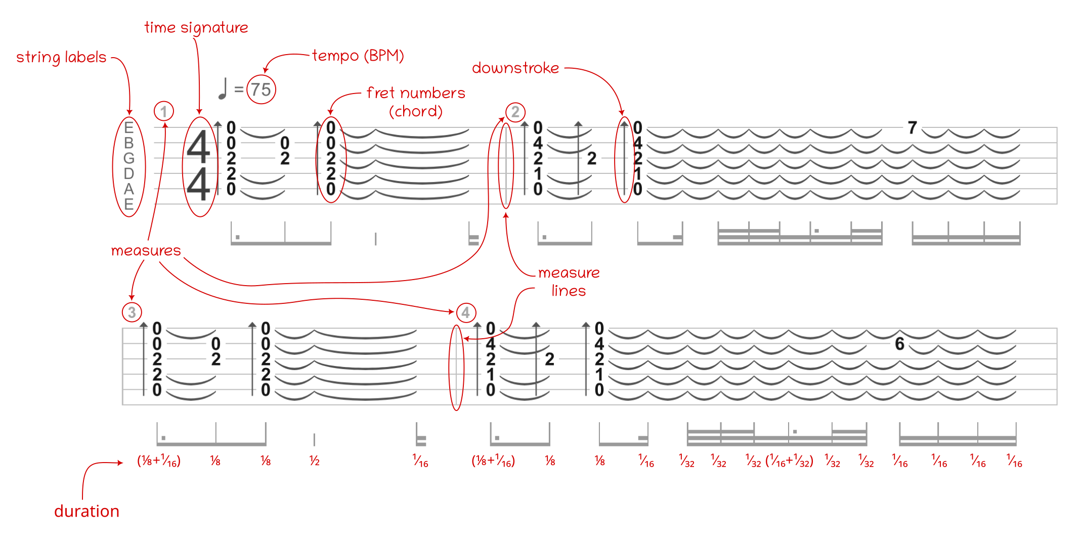
The tablature above begins with string labels corresponding to the guitar’s standard tuning, the ⁴⁄₄ time signature, and a seventy-five beats per minute tempo. Each measure is numbered and separated from its neighbors by a vertical line to help you orient yourself as you read through the music.
The bolded numbers that appear on the horizontal lines indicate the frets you should press on the corresponding strings to sound the desired chord. Finally, the symbols below each measure represent the fractional duration of notes and rests (pauses) relative to the whole note.
Note: Check out Songsterr’s official help page for more information on how to read a tab on their website.
Based on this knowledge, you can interpret the provided tab and breathe life into it with the help of the guitar synthesizer that you’ve implemented. Initially, you’ll hard code the Diablo guitar tab in a Python script using a programmatic approach.
Play Diablo Tablature Programmatically
Create a new script called play_diablo.py in the demo/ folder with the following content:
demo/play_diablo.py
from fractions import Fraction

from digitar.temporal import Time

BEATS_PER_MINUTE = 75
BEATS_PER_MEASURE = 4
NOTE_VALUE = Fraction(1, 4)

class MeasureTiming:
    BEAT = Time(seconds=60 / BEATS_PER_MINUTE)
    MEASURE = BEAT * BEATS_PER_MEASURE

class Note:
    WHOLE = MeasureTiming.BEAT * NOTE_VALUE.denominator
    SEVEN_SIXTEENTH = WHOLE * Fraction(7, 16)
    FIVE_SIXTEENTH = WHOLE * Fraction(5, 16)
    THREE_SIXTEENTH = WHOLE * Fraction(3, 16)
    ONE_EIGHTH = WHOLE * Fraction(1, 8)
    ONE_SIXTEENTH = WHOLE * Fraction(1, 16)
    ONE_THIRTY_SECOND = WHOLE * Fraction(1, 32)

class StrummingSpeed:
    SLOW = Time.from_milliseconds(40)
    FAST = Time.from_milliseconds(20)
    SUPER_FAST = Time.from_milliseconds(5)
The highlighted constants represent the only input parameters that you can change, while the remaining values are derived from those inputs. Here, you group logically related values under common namespaces by defining them as class attributes. The respective class names tell you their purpose.
Note: Your immediate instinct might tell you to use Python’s Enum data type to group constants. But, in this case, you’re interested in the underlying values rather than the enumeration members that wrap them. Moreover, with an Enum, you wouldn’t be able to base the individual note values on the WHOLE note, which you compute dynamically. Finally, the BEAT and MEASURE don’t constitute mutually exclusive choices.
Next, define your virtual guitar, hook it up to the synthesizer, and prepare the audio track along with the timeline that’s aware of the tab measures:
demo/play_diablo.py
from fractions import Fraction

from pedalboard.io import AudioFile

from digitar.instrument import PluckedStringInstrument, StringTuning
from digitar.processing import normalize
from digitar.synthesis import Synthesizer
from digitar.temporal import MeasuredTimeline, Time
from digitar.track import AudioTrack

# ...

def main() -> None:
    acoustic_guitar = PluckedStringInstrument(
        tuning=StringTuning.from_notes("E2", "A2", "D3", "G3", "B3", "E4"),
        vibration=Time(seconds=10),
        damping=0.498,
    )
    synthesizer = Synthesizer(acoustic_guitar)
    audio_track = AudioTrack(synthesizer.sampling_rate)
    timeline = MeasuredTimeline(measure=MeasureTiming.MEASURE)
    save(audio_track, "diablo.mp3")

def save(audio_track: AudioTrack, filename: str) -> None:
    with AudioFile(filename, "w", audio_track.sampling_rate) as file:
        file.write(normalize(audio_track.samples))
    print(f"\nSaved file {filename!r}")

if __name__ == "__main__":
    main()
You reuse the acoustic guitar object from previous sections, which applies the standard tuning, and you define a helper function to save the resulting audio in a file.
Note: Be careful when you pass the measure size into a MeasuredTimeline instance. If you passed it as a positional argument rather than a keyword argument, then you’d initialize the .instant field instead of the intended .measure one.
What you’ll put on the timeline are synthesized sounds described by the current instant, the fret numbers to press, and the stroke velocity, which you can model as an immutable data class:
demo/play_diablo.py
from dataclasses import dataclass
from fractions import Fraction

from pedalboard.io import AudioFile

from digitar.chord import Chord
from digitar.instrument import PluckedStringInstrument, StringTuning
from digitar.processing import normalize
from digitar.stroke import Velocity
from digitar.synthesis import Synthesizer
from digitar.temporal import MeasuredTimeline, Time
from digitar.track import AudioTrack

# ...

@dataclass(frozen=True)
class Stroke:
    instant: Time
    chord: Chord
    velocity: Velocity

# ...
Objects of the Stroke class represent precisely what you see on the guitar tab provided by Songsterr. You can now translate each measure into a sequence of strokes to loop through:
demo/play_diablo.py
# ...

def main() -> None:
    acoustic_guitar = PluckedStringInstrument(
        tuning=StringTuning.from_notes("E2", "A2", "D3", "G3", "B3", "E4"),
        vibration=Time(seconds=10),
        damping=0.498,
    )
    synthesizer = Synthesizer(acoustic_guitar)
    audio_track = AudioTrack(synthesizer.sampling_rate)
    timeline = MeasuredTimeline(measure=MeasureTiming.MEASURE)
    for measure in measures(timeline):
        for stroke in measure:
            audio_track.add_at(
                stroke.instant,
                synthesizer.strum_strings(stroke.chord, stroke.velocity),
            )
    save(audio_track, "diablo.mp3")

def measures(timeline: MeasuredTimeline) -> tuple[tuple[Stroke, ...], ...]:
    return (
        measure_01(timeline),
        measure_02(timeline),
    )

# ...
First, you iterate over a sequence of measures returned by your measures() function, which you call with the timeline as an argument. Then, you iterate over each stroke within the current measure, synthesize the corresponding chord, and add it to the track at the right moment.
Your guitar tab currently contains two measures, each computed in a separate function, which you can define now:
demo/play_diablo.py
# ...

def measure_01(timeline: MeasuredTimeline) -> tuple[Stroke, ...]:
    return (
        Stroke(
            timeline.instant,
            Chord.from_numbers(0, 0, 2, 2, 0, None),
            Velocity.down(StrummingSpeed.SLOW),
        ),
        Stroke(
            (timeline >> Note.THREE_SIXTEENTH).instant,
            Chord.from_numbers(None, 0, 2, None, None, None),
            Velocity.up(StrummingSpeed.FAST),
        ),
        Stroke(
            (timeline >> Note.ONE_EIGHTH).instant,
            Chord.from_numbers(0, 0, 2, 2, 0, None),
            Velocity.down(StrummingSpeed.SLOW),
        ),
    )

def measure_02(timeline: MeasuredTimeline) -> tuple[Stroke, ...]:
    return (
        Stroke(
            next(timeline).instant,
            Chord.from_numbers(0, 4, 2, 1, 0, None),
            Velocity.down(StrummingSpeed.SLOW),
        ),
        Stroke(
            (timeline >> Note.THREE_SIXTEENTH).instant,
            Chord.from_numbers(None, None, 2, None, None, None),
            Velocity.down(StrummingSpeed.SUPER_FAST),
        ),
        Stroke(
            (timeline >> Note.ONE_EIGHTH).instant,
            Chord.from_numbers(0, 4, 2, 1, 0, None),
            Velocity.down(StrummingSpeed.SLOW),
        ),
        Stroke(
            (timeline >> Note.SEVEN_SIXTEENTH).instant,
            Chord.from_numbers(7, None, None, None, None, None),
            Velocity.down(StrummingSpeed.SUPER_FAST),
        ),
    )

# ...
The complete Diablo guitar tab has seventy-eight measures with over a thousand strokes in total. For brevity, the code snippet above only shows the first two measures, which should be enough to recognize the famous theme. While it’ll suffice for the sake of the example, feel free to implement the subsequent measures based on the Songsterr tab.
Alternatively, you can copy the final source code of the remaining functions from the bonus materials. To get them, click the link below:
Get Your Code: Click here to download the free sample code that you’ll use to build a guitar synthesizer in Python.
Beware that the full play_diablo.py script contains several thousand lines of Python code! Therefore, you might find it more convenient to continue working on this minimal viable prototype for the time being.
Notice that each stroke, except for the very first one, shifts the timeline by a fraction of the whole note to reflect the duration of the previous chord. This ensures the correct spacing between adjacent chords. Additionally, the highlighted line moves the timeline to the beginning of the next measure in the tab.
In total, there are six unique fractional notes that you’ll need for the Diablo soundtrack. When you know the whole note’s duration in seconds, you can quickly infer the durations of the remaining notes:
| Note | Seconds | Fraction |
|---|---|---|
| Whole | 3.2s | 1 |
| Seven-sixteenth | 1.4s | ⁷⁄₁₆ = (¹⁄₁₆ + ⅛ + ¼) |
| Five-sixteenth | 1.0s | ⁵⁄₁₆ = (¹⁄₁₆ + ¼) |
| Three-sixteenth | 0.6s | ³⁄₁₆ = (¹⁄₁₆ + ⅛) |
| One-eighth | 0.4s | ⅛ |
| One-sixteenth | 0.2s | ¹⁄₁₆ |
| One-thirty-second | 0.1s | ¹⁄₃₂ |
Assuming that the whole note has the same duration as the entire measure, 3.2 seconds, then a one-thirty-second note is 0.1 seconds, and so on. The division of the whole note’s duration allows you to piece together the rhythm of the soundtrack with great accuracy.
Wouldn’t it be great to create a universal player that can read and synthesize any guitar tab instead of just this particular one? You’ll eventually get there, but before that, you’ll refine the synthesis to make it sound even more authentic.
Step 6: Apply Special Effects for More Realism
At this point, your guitar synthesizer does a pretty good job of simulating a real instrument, but it still sounds a bit harsh and artificial. There are many ways to enhance the timbre of the virtual guitar, but in this section, you’ll limit yourself to the special effects provided by the Pedalboard library. It lets you chain several effects together, just like a genuine guitar pedalboard operated by foot.
Boost the Bass and Add a Reverberation Effect
A real guitar has a sound box, which produces a rich and vibrant sound toward the lower frequencies. To mimic this in your virtual guitar and amplify the bass, you can use an audio equalizer (EQ). Additionally, by adding a reverberation effect, you’ll simulate the natural echo and decay that occurs in a physical space, giving the sound more depth and realism.
While Pedalboard doesn’t include a dedicated equalizer, you can combine various audio plugins to achieve the desired effect. Modify your play_diablo.py script by applying a reverb, low shelf filter, and gain to the synthesized audio track:
demo/play_diablo.py
from dataclasses import dataclass
from fractions import Fraction

import numpy as np
from pedalboard import Gain, LowShelfFilter, Pedalboard, Reverb
from pedalboard.io import AudioFile

from digitar.chord import Chord
from digitar.instrument import PluckedStringInstrument, StringTuning
from digitar.processing import normalize
from digitar.stroke import Velocity
from digitar.synthesis import Synthesizer
from digitar.temporal import MeasuredTimeline, Time
from digitar.track import AudioTrack

# ...

def save(audio_track, filename):
    with AudioFile(filename, "w", audio_track.sampling_rate) as file:
        file.write(normalize(apply_effects(audio_track)))
    print(f"\nSaved file {filename!r}")

def apply_effects(audio_track: AudioTrack) -> np.ndarray:
    effects = Pedalboard([
        Reverb(),
        LowShelfFilter(cutoff_frequency_hz=440, gain_db=10, q=1),
        Gain(gain_db=6),
    ])
    return effects(audio_track.samples, audio_track.sampling_rate)

if __name__ == "__main__":
    main()
First, you import the corresponding plugins from the library and use them to build a virtual pedalboard. Once assembled, you call it on the audio track and normalize the resulting samples before saving them in a file.
The reverb relies on the default settings, while the low shelf filter is set with a cutoff frequency of 440 Hz, a gain of 10 dB, and a Q factor of 1. The gain is set to increase the volume by 6 dB. You can experiment with different parameter values to tailor the sound to your liking or to better fit a particular music genre.
When you run the script again and play the resulting audio file, you should hear a more natural sound. Your digital guitar is starting to resemble the tone of an acoustic guitar. However, there’s one particular effect that can make a real difference, and you’re going to explore it now.
Apply a Convolution Reverb Filter With an IR
The idea behind a convolution reverb is to simulate the reverberation of a physical space through a filter that employs an impulse response (IR). An impulse response is a recording of the acoustic characteristics of a real-world location, such as a concert hall, church, or small room. It’s usually a short sound like a clap or a balloon pop, which captures how a space responds to a full spectrum of frequencies.
With this special type of reverb, you can record vocals in a studio, for example, and apply the ambience of a grand cathedral in post-production. You’ll get the impression that the performance was actually recorded in that exact location. Check out the Open AIR library for a collection of high-quality impulse responses from various places around the world. You can listen to and compare the before and after versions. The difference is remarkable!
In the context of guitars, impulse responses can help you emulate the sound of different guitar amplifiers or even model the sound of specific instruments, such as a banjo or ukulele. The filter convolves your unprocessed or dry signal with the impulse response, effectively imprinting the acoustic characteristics of the original instrument onto the audio. This creates a highly realistic effect, adding depth and character to your digital guitar.
Open the play_diablo.py script again and insert a convolution filter with a path to the impulse response file of an acoustic guitar:
demo/play_diablo.py
from dataclasses import dataclass
from fractions import Fraction

import numpy as np
from pedalboard import Convolution, Gain, LowShelfFilter, Pedalboard, Reverb
from pedalboard.io import AudioFile

# ...

def apply_effects(audio_track: AudioTrack) -> np.ndarray:
    effects = Pedalboard([
        Reverb(),
        Convolution(impulse_response_filename="ir/acoustic.wav", mix=0.95),
        LowShelfFilter(cutoff_frequency_hz=440, gain_db=10, q=1),
        Gain(gain_db=6),
    ])
    return effects(audio_track.samples, audio_track.sampling_rate)

if __name__ == "__main__":
    main()
There are lots of free impulse responses for guitars online. However, finding one that’s good quality can be a bit of a challenge. The impulse response files used in this tutorial come from these sources:
| Instrument | Filename |
|---|---|
| Acoustic Guitar | Tay816 M251 SB1.wav |
| Bass Guitar | Holy Grail C800 SB1.wav |
| Electric Guitar | Rocksta Reactions Mesa Traditional D6 D 0 -18 -36.wav |
| Banjo | IR_5_string_banjo_dazzo_IR44k |
| Ukulele | AtlasV2.wav |
You can follow the links above to find the corresponding sample packs. Alternatively, download this tutorial’s supporting materials, which include conveniently named individual impulse response files. Once you’ve downloaded those files, place them under the ir/ subfolder where you keep your demo scripts:
digital-guitar/
│
├── demo/
│   ├── ir/
│   │   ├── acoustic.wav
│   │   ├── banjo.wav
│   │   ├── bass.wav
│   │   ├── electric.wav
│   │   └── ukulele.wav
│   │
│   ├── play_chorus.py
│   └── play_diablo.py
│
└── (...)
You can now update your other script, play_chorus.py, by applying similar effects and using the corresponding impulse response to enhance the synthesized sound:
demo/play_chorus.py
from itertools import cycle
from typing import Iterator

from pedalboard import Convolution, Gain, LowShelfFilter, Pedalboard, Reverb
from pedalboard.io import AudioFile

# ...

def main() -> None:
    ukulele = PluckedStringInstrument(
        tuning=StringTuning.from_notes("A4", "E4", "C4", "G4"),
        vibration=Time(seconds=5.0),
        damping=0.498,
    )
    synthesizer = Synthesizer(ukulele)
    audio_track = AudioTrack(synthesizer.sampling_rate)
    timeline = Timeline()
    for interval, chord, stroke in strumming_pattern():
        audio_samples = synthesizer.strum_strings(chord, stroke)
        audio_track.add_at(timeline.instant, audio_samples)
        timeline >> interval
    effects = Pedalboard(
        [
            Reverb(),
            Convolution(impulse_response_filename="ir/ukulele.wav", mix=0.95),
            LowShelfFilter(cutoff_frequency_hz=440, gain_db=10, q=1),
            Gain(gain_db=15),
        ]
    )
    samples = effects(audio_track.samples, audio_track.sampling_rate)
    with AudioFile("chorus.mp3", "w", audio_track.sampling_rate) as file:
        file.write(normalize(samples))

# ...
Again, you can play around with these parameters or even try out different plugins from the Pedalboard library.
Okay. So far, you’ve modeled an acoustic guitar and a ukulele. How about playing an electric guitar or a bass guitar this time? As you’re about to witness, simulating these instruments mostly boils down to choosing the right effects from the plugin library and tweaking the string tuning and vibration time. To avoid code duplication and repetition, you’ll keep the chords in a separate file from now on.
Step 7: Load Guitar Tablature From a File
There are numerous guitar tablature data formats out there, ranging from simple ASCII tab to more complex binary formats like Power Tab or Guitar Pro. Some of them require specialized or proprietary software to read. In this section, you’ll devise your own file format to represent the most essential features of the tabs hosted on the Songsterr website. At the end, you’ll top it off with a dedicated tablature player so you can hear the music!
Design the File Format for Your Guitar Tabs
Before writing a single line of code, take a step back and consider how you want to use your new guitar tab format. In particular, what kind of information do you want the tab to include, and how do you plan to present it?
Below are the suggested design goals for your custom format, which should be:
- Human-Readable: The format must be legible for humans so that you can edit the tabs in a plain text editor.
- Intuitive: You want the format to have a familiar syntax and a gentle learning curve to make you feel at home as quickly as possible.
- Concise: Most songs repeat the same chords and patterns throughout, so the format should efficiently represent them to avoid unnecessary verbosity.
- Hierarchical: The format should have a hierarchical structure, allowing for convenient deserialization to a Python dictionary.
- Multi-Track: A single tab file should allow you to store one or more tracks that correspond to virtual instruments and mix them in various proportions.
When you consider these requirements, then XML, JSON, and YAML emerge as the top candidates for the underlying data format on which you can build. All are text-based, widely known, and have a hierarchical structure, letting you put multiple tracks in them. That said, only YAML ticks all the boxes, as you can’t easily avoid repetition with the other two formats.
YAML is also a good choice because it supports anchors and aliases, which let you reuse repeated elements without having to rewrite them. That can save you a lot of typing, especially in the context of guitar tabs!
Have a look at an excerpt of a fictional guitar tab below, which demonstrates some of your format’s features:
 1title: Hello, World!  # Optional
 2artist: John Doe  # Optional
 3tracks:
 4  acoustic:  # Arbitrary name
 5    url: https://www.songsterr.com/hello  # Optional
 6    weight: 0.8  # Optional (defaults to 1.0)
 7    instrument:
 8      tuning: [E2, A2, D3, G3, B3, E4]
 9      vibration: 5.5
10      damping: 0.498  # Optional (defaults to 0.5)
11      effects:  # Optional
12      - Reverb
13      - Convolution:
14          impulse_response_filename: acoustic.wav
15          mix: 0.95
16    tablature:
17      beats_per_minute: 75
18      measures:
19      - time_signature: 4/4
20        notes:  # Optional (can be empty measure)
21        - frets: [0, 0, 2, 2, 0, ~]
22          offset: 1/8  # Optional (defaults to zero)
23          upstroke: true  # Optional (defaults to false)
24          arpeggio: 0.04  # Optional (defaults to 0.005)
25          vibration: 3.5  # Optional (overrides instrument's defaults)
26      - time_signature: 4/4
27      - time_signature: 4/4
28        notes: &loop
29        - frets: &seven [~, ~, ~, ~, 7, ~]
30        - frets: *seven
31          offset: 1/4
32        - frets: *seven
33          offset: 1/4
34        - frets: *seven
35          offset: 1/4
36      - time_signature: 4/4
37        notes: *loop
38      # ...
39  electric:
40    # ...
41  ukulele:
42    # ...
Many of the attributes are completely optional, and most have sensible default values, including:
- Weight: The tracks in your tab will be mixed with a weight of one unless you explicitly request a different weight.
- Damping: If you don’t specify the instrument’s damping, then it’ll default to 0.5, which represents a simple average.
- Notes: You can skip the notes to signify an empty measure, which sometimes makes sense when you want to synchronize a few instruments.
- Offset: When you don’t specify an offset, the corresponding note or chord will be placed at whatever the current position is on the timeline. You’ll typically omit the offset of the first note in a measure unless it doesn’t occur on the beat.
- Upstroke: Most strokes are directed down, so you must only set this attribute when you want the chord to be strummed upward.
- Arpeggio: The stroke’s velocity or the delay between the individual plucks in a chord assumes five milliseconds by default, which is fairly quick.
- Vibration: You only ever need to set the note’s vibration if you want to override the default string vibration defined in the respective instrument.
The optional effects of an instrument represent Pedalboard plugins. You can chain them in a specific order to create the desired outcome, or you can skip them altogether. Each effect must be either a plugin’s class name or a mapping of the class name to the corresponding constructor’s arguments. You can check out Pedalboard’s documentation for more details on how to configure these effects.
Each track has its own tablature consisting of the tempo—expressed as the number of beats per second—and a list of measures. In turn, each measure provides a time signature and a list of notes or chords. A single note must define at least the fret numbers to press down, as the rest of the attributes are optional. However, most note instances will also specify the offset in terms of a fraction of the whole note.
Note: In YAML, you can use the tilde character (~) to represent the lack of a value, which is more compact than writing out null. Plus, when you squint your eyes, the tilde resembles a dash character from the ASCII tab format.
Anchors and aliases are two of the most powerful features of YAML. They let you define a value once and bind it to a global variable in the document. Variable names must start with the ampersand character (&), and you can reference them by using the asterisk (*) instead of the ampersand. If you’ve done any C programming, then this is analogous to taking the address of a variable and dereferencing a pointer, respectively.
In the example above, you declare two global variables or YAML anchors:
&seven: Represents the fret numbers, which repeat throughout the measure&loop: Captures the measure itself, allowing you to use the same loop many times in the composition
This not only saves space and typing but also makes the document more maintainable. If you want to change the sequence, then you only need to update it in one place, and the change will be reflected wherever you used the alias.
Having seen a sample guitar tab in your YAML-based file format, you can now load it into Python. You’ll accomplish this with the help of the Pydantic library.
Define Pydantic Models to Load From YAML
Create a sibling package named tablature next to digitar that you created before. When you do this, you should end up with the following folder structure:
digital-guitar/
│
├── demo/
│   ├── ir/
│   │   └── (...)
│   │
│   ├── play_chorus.py
│   └── play_diablo.py
│
├── src/
│   ├── digitar/
│   │    ├── __init__.py
│   │    ├── burst.py
│   │    ├── chord.py
│   │    ├── instrument.py
│   │    ├── pitch.py
│   │    ├── processing.py
│   │    ├── stroke.py
│   │    ├── synthesis.py
│   │    ├── temporal.py
│   │    └── track.py
│   │
│   └── tablature/
│       └── __init__.py
│
├── tests/
│   └── __init__.py
│
├── pyproject.toml
└── README.md
Now, create a Python module named models and place it in the new package. This module will contain the Pydantic model classes for your YAML-based data format. Start by modeling the root element of the document, which you’ll call Song:
src/tablature/models.py
from pathlib import Path
from typing import Optional, Self

import yaml
from pydantic import BaseModel

class Song(BaseModel):
    title: Optional[str] = None
    artist: Optional[str] = None
    tracks: dict[str, Track]

    @classmethod
    def from_file(cls, path: str | Path) -> Self:
        with Path(path).open(encoding="utf-8") as file:
            return cls(**yaml.safe_load(file))
The document’s root element has two optional attributes, .title and .artist, as well as a mandatory .tracks dictionary. The latter maps arbitrary track names to Track instances, which you’ll implement in a bit. The class also provides a method for loading YAML documents from a file indicated by either a string or a Path instance and deserializing them into the model object.
Because Python reads your source code from top to bottom, you’ll need to define the Track before your Song model, which depends on it:
src/tablature/models.py
from pathlib import Path
from typing import Optional, Self

import yaml
from pydantic import BaseModel, HttpUrl, NonNegativeFloat, model_validator

class Track(BaseModel):
    url: Optional[HttpUrl] = None
    weight: Optional[NonNegativeFloat] = 1.0
    instrument: Instrument
    tablature: Tablature

    @model_validator(mode="after")
    def check_frets(self) -> Self:
        num_strings = len(self.instrument.tuning)
        for measure in self.tablature.measures:
            for notes in measure.notes:
                if len(notes.frets) != num_strings:
                    raise ValueError("Incorrect number of frets")
        return self

class Song(BaseModel):
    # ...
A Track instance consists of a pair of optional attributes , .url and .weight, and a pair of required attributes, .instrument and .tablature. The weight represents the track’s relative volume in the final mix. The decorated method, .check_frets(), validates if the number of frets in each measure matches the number of strings in the instrument.
The Instrument model reflects your digitar.PluckedStringInstrument type, augmenting it with a chain of Pedalboard plugins:
src/tablature/models.py
from pathlib import Path
from typing import Optional, Self

import yaml
from pydantic import (BaseModel, HttpUrl, NonNegativeFloat, PositiveFloat,
                      confloat, conlist, constr, model_validator)

DEFAULT_STRING_DAMPING: float = 0.5

class Instrument(BaseModel):
    tuning: conlist(constr(pattern=r"([A-G]#?)(-?\d+)?"), min_length=1)
    vibration: PositiveFloat
    damping: Optional[confloat(ge=0, le=0.5)] = DEFAULT_STRING_DAMPING
    effects: Optional[tuple[str | dict, ...]] = tuple()

class Track(BaseModel):
    # ...

class Song(BaseModel):
    # ...
The .tuning attribute is a list of at least one element constrained to the string data type matching the regular expression of a musical note in scientific pitch notation. The .vibration represents how long in seconds the instrument’s strings should vibrate by default. You can override this value per stroke if you need to. The .damping is a floating-point value restricted to the specified interval and defaulting to a value stored in a constant.
Your next model, Tablature, consists of only two attributes:
src/tablature/models.py
from pathlib import Path
from typing import Optional, Self

import yaml
from pydantic import (BaseModel, HttpUrl, NonNegativeFloat, PositiveFloat,
                      PositiveInt, confloat, conlist, constr, model_validator)

DEFAULT_STRING_DAMPING: float = 0.5

class Tablature(BaseModel):
    beats_per_minute: PositiveInt
    measures: tuple[Measure, ...]

class Instrument(BaseModel):
    # ...

class Track(BaseModel):
    # ...

class Song(BaseModel):
    # ...
Both .beats_per_minute and .measures are obligatory. The first attribute is a positive integer indicating the tempo of the song in beats per minute. The second attribute is a tuple containing one or more Measure objects, which you can implement now:
src/tablature/models.py
from fractions import Fraction
from functools import cached_property
from pathlib import Path
from typing import Optional, Self

import yaml
from pydantic import (BaseModel, HttpUrl, NonNegativeFloat, PositiveFloat,
                      PositiveInt, confloat, conlist, constr, model_validator)

DEFAULT_STRING_DAMPING: float = 0.5

class Measure(BaseModel):
    time_signature: constr(pattern=r"\d+/\d+")
    notes: Optional[tuple[Note, ...]] = tuple()

    @cached_property
    def beats_per_measure(self) -> int:
        return int(self.time_signature.split("/")[0])

    @cached_property
    def note_value(self) -> Fraction:
        return Fraction(1, int(self.time_signature.split("/")[1]))

class Tablature(BaseModel):
    # ...

class Instrument(BaseModel):
    # ...

class Track(BaseModel):
    # ...

class Song(BaseModel):
    # ...
Each Measure is allowed to specify its own .time_signature with a fractional notation, such as 4/4. The .notes tuple is optional because a measure can be empty. The two cached properties extract the number of beats within a measure and the note value from the time signature.
Finally, you can write down your last model representing a note or chord to play on the virtual guitar:
src/tablature/models.py
from fractions import Fraction
from functools import cached_property
from pathlib import Path
from typing import Optional, Self

import yaml
from pydantic import (BaseModel, HttpUrl, NonNegativeFloat, NonNegativeInt,
                      PositiveFloat, PositiveInt, confloat, conlist, constr,
                      model_validator)

DEFAULT_STRING_DAMPING: float = 0.5
DEFAULT_ARPEGGIO_SECONDS: float = 0.005

class Note(BaseModel):
    frets: conlist(NonNegativeInt | None, min_length=1)
    offset: Optional[constr(pattern=r"\d+/\d+")] = "0/1"
    upstroke: Optional[bool] = False
    arpeggio: Optional[NonNegativeFloat] = DEFAULT_ARPEGGIO_SECONDS
    vibration: Optional[PositiveFloat] = None

class Measure(BaseModel):
    # ...

class Tablature(BaseModel):
    # ...

class Instrument(BaseModel):
    # ...

class Track(BaseModel):
    # ...

class Song(BaseModel):
    # ...
This model has only one required attribute, .frets, which is a list of fret numbers constrained to either None or non-negative integer elements. The .offset of a note must be given as a fraction of the whole note, such as 1/8. Otherwise, it defaults to zero. The remaining attributes include .upstroke, .arpeggio, and .vibration, which describe how to play the stroke.
With these models, you can load the guitar tablature examples provided in the supporting materials. For instance, one of the included YAML files is based on a Songsterr tab for the Foggy Mountain Breakdown by Earl Scruggs, featuring a banjo, an acoustic guitar, and a bass guitar:
>>> from tablature.models import Song

>>> song = Song.from_file("demo/tabs/foggy-mountain-breakdown.yaml")
>>> sorted(song.tracks)
['acoustic', 'banjo', 'bass']

>>> banjo = song.tracks["banjo"].instrument
>>> banjo.tuning
['G4', 'D3', 'G3', 'B3', 'D4']

>>> banjo_tab = song.tracks["banjo"].tablature
>>> banjo_tab.measures[-1].notes
(
    Note(
        frets=[None, None, 0, None, None],
        offset='0/1',
        upstroke=False,
        arpeggio=0.005,
        vibration=None
    ),
    Note(
        frets=[0, None, None, None, 0],
        offset='1/2',
        upstroke=False,
        arpeggio=0.005,
        vibration=None
    )
)
You read a YAML file with the guitar tablature and deserialize it into a hierarchy of Pydantic models. Then, you access the track associated with the banjo tablature and display the notes in its last measure.
Next up, you’ll build a player that can take these models, translate them into your digital guitar domain, and spit out a synthesized audio file. Are you ready for the challenge?
Implement the Guitar Tablature Reader
Define a scripts section in your pyproject.toml file with an entry point to your Python project, which you’ll later run from the command line:
pyproject.toml
# ...

[tool.poetry.scripts]
play-tab = "tablature.player:main"
This defines the play-tab command pointing to a new module named player in the tablature package. You can scaffold that module now by implementing these few functions in it:
src/tablature/player.py
from argparse import ArgumentParser, Namespace
from pathlib import Path

from tablature import models

SAMPLING_RATE = 44100

def main() -> None:
    play(parse_args())

def parse_args() -> Namespace:
    parser = ArgumentParser()
    parser.add_argument("path", type=Path, help="tablature file (.yaml)")
    parser.add_argument("-o", "--output", type=Path, default=None)
    return parser.parse_args()

def play(args: Namespace) -> None:
    song = models.Song.from_file(args.path)
The main() function is what Poetry will call when you invoke poetry run play-tab in your terminal. This function parses command-line arguments using argparse and passes them to the play() function, which loads a song from the specified YAML file through your Pydantic model.
You must specify the path to the guitar tablature as a positional argument, and you can provide the path to the output audio file as an option. If you don’t, then the resulting file will share its base name with your input file.
Once you have the tab loaded into Python, you can interpret it by synthesizing the individual tracks:
src/tablature/player.py
from argparse import ArgumentParser, Namespace
from pathlib import Path

import numpy as np
from digitar.instrument import PluckedStringInstrument, StringTuning
from digitar.synthesis import Synthesizer
from digitar.temporal import MeasuredTimeline, Time
from digitar.track import AudioTrack

from tablature import models

# ...

def play(args: Namespace) -> None:
    song = models.Song.from_file(args.path)
    tracks = [
        track.weight * synthesize(track)
        for track in song.tracks.values()
    ]

def synthesize(track: models.Track) -> np.ndarray:
    synthesizer = Synthesizer(
        instrument=PluckedStringInstrument(
            tuning=StringTuning.from_notes(*track.instrument.tuning),
            damping=track.instrument.damping,
            vibration=Time(track.instrument.vibration),
        ),
        sampling_rate=SAMPLING_RATE,
    )
    audio_track = AudioTrack(synthesizer.sampling_rate)
    timeline = MeasuredTimeline()
    read(track.tablature, synthesizer, audio_track, timeline)
    return apply_effects(audio_track, track.instrument)
You use a list comprehension to synthesize each track and multiply the resulting NumPy array of samples by the track’s weight.
The synthesize() function creates a synthesizer object based on the instrument definition in the track. It then reads the corresponding tablature, placing notes on the timeline. Finally, it applies special effects with Pedalboard before returning the audio samples to the caller.
The read() function automates the manual steps that you previously carried out when you played the Diablo tab programmatically:
src/tablature/player.py
from argparse import ArgumentParser, Namespace
from fractions import Fraction
from pathlib import Path

import numpy as np
from digitar.chord import Chord
from digitar.instrument import PluckedStringInstrument, StringTuning
from digitar.stroke import Velocity
from digitar.synthesis import Synthesizer
from digitar.temporal import MeasuredTimeline, Time
from digitar.track import AudioTrack

from tablature import models

# ...

def read(
    tablature: models.Tablature,
    synthesizer: Synthesizer,
    audio_track: AudioTrack,
    timeline: MeasuredTimeline,
) -> None:
    beat = Time(seconds=60 / tablature.beats_per_minute)
    for measure in tablature.measures:
        timeline.measure = beat * measure.beats_per_measure
        whole_note = beat * measure.note_value.denominator
        for note in measure.notes:
            stroke = Velocity.up if note.upstroke else Velocity.down
            audio_track.add_at(
                (timeline >> (whole_note * Fraction(note.offset))).instant,
                synthesizer.strum_strings(
                    chord=Chord(note.frets),
                    velocity=stroke(delay=Time(note.arpeggio)),
                    vibration=(
                        Time(note.vibration) if note.vibration else None
                    ),
                ),
            )
        next(timeline)
It starts by finding the beat duration in seconds. Based on that, the function calculates the duration of the current measure and the whole note in the tab. Next, it iterates through each note in the measure, synthesizes the corresponding chord, and adds it to the audio track at the calculated time. After each iteration, the function calls next() on the timeline in order to advance it to the next measure.
The following three functions work in tandem to import and apply the desired plugins from the Pedalboard library based on the declarations in the YAML file:
src/tablature/player.py
from argparse import ArgumentParser, Namespace
from fractions import Fraction
from pathlib import Path

import numpy as np
import pedalboard

# ...

def apply_effects(
    audio_track: AudioTrack, instrument: models.Instrument
) -> np.ndarray:
    effects = pedalboard.Pedalboard(get_plugins(instrument))
    return effects(audio_track.samples, audio_track.sampling_rate)

def get_plugins(instrument: models.Instrument) -> list[pedalboard.Plugin]:
    return [get_plugin(effect) for effect in instrument.effects]

def get_plugin(effect: str | dict) -> pedalboard.Plugin:
    match effect:
        case str() as class_name:
            return getattr(pedalboard, class_name)()
        case dict() as plugin_dict if len(plugin_dict) == 1:
            class_name, params = list(plugin_dict.items())[0]
            return getattr(pedalboard, class_name)(**params)
The first function applies the effects associated with a specific instrument to an audio track. It creates a Pedalboard object from the plugins retrieved from the track’s instrument. The last function returns a plugin instance based on its name and optionally initializes it with the parameters specified in the tablature document.
Now, you can mix your synthesized tracks and save them in a file. To do that, you’ll need to modify the play() function:
src/tablature/player.py
from argparse import ArgumentParser, Namespace
from fractions import Fraction
from pathlib import Path

import numpy as np
import pedalboard
from digitar.chord import Chord
from digitar.instrument import PluckedStringInstrument, StringTuning
from digitar.processing import normalize
from digitar.stroke import Velocity
from digitar.synthesis import Synthesizer
from digitar.temporal import MeasuredTimeline, Time
from digitar.track import AudioTrack
from pedalboard.io import AudioFile

from tablature import models

# ...

def play(args: Namespace) -> None:
    song = models.Song.from_file(args.path)
    samples = normalize(
        np.sum(
            pad_to_longest(
                [
                    track.weight * synthesize(track)
                    for track in song.tracks.values()
                ]
            ),
            axis=0,
        )
    )
    save(
        samples,
        args.output or Path.cwd() / args.path.with_suffix(".mp3").name,
    )

def pad_to_longest(tracks: list[np.ndarray]) -> list[np.ndarray]:
    max_length = max(array.size for array in tracks)
    return [
        np.pad(array, (0, max_length - array.size)) for array in tracks
    ]

def save(samples: np.ndarray, path: Path) -> None:
    with AudioFile(str(path), "w", SAMPLING_RATE) as file:
        file.write(samples)
    print(f"Saved file {path.absolute()}")

# ...
Because the individual tracks may differ in length, you pad them to ensure they’re all the same length before adding their amplitudes with np.sum() and normalizing their values. Lastly, you save the audio samples to a file by calling your save() function.
However, to ensure that relative paths within your YAML document will work as expected, you should temporarily change the script’s current working directory:
src/tablature/player.py
import os
from argparse import ArgumentParser, Namespace
from contextlib import contextmanager
from fractions import Fraction
from pathlib import Path

# ...

def play(args: Namespace) -> None:
    song = models.Song.from_file(args.path)
    with chdir(args.path.parent):
        samples = normalize(
            np.sum(
                pad_to_longest(
                    [
                        track.weight * synthesize(track)
                        for track in song.tracks.values()
                    ]
                ),
                axis=0,
            )
        )
    save(
        samples,
        args.output or Path.cwd() / args.path.with_suffix(".mp3").name,
    )

@contextmanager
def chdir(directory: Path) -> None:
    current_dir = os.getcwd()
    os.chdir(directory)
    try:
        yield
    finally:
        os.chdir(current_dir)

# ...
You specify a function-based context manager that you call using the with statement to set the working directory to the YAML file’s parent folder. Without it, you wouldn’t be able to find and load the impulse response files for the Pedalboard’s convolution plugin.
Okay. Below is how you can use the play-tab script in the terminal. Don’t forget to reinstall your Poetry project to make the entry point defined in pyproject.toml take effect:
$ poetry install
$ poetry run play-tab demo/tabs/foggy-mountain-breakdown.yaml -o foggy.mp3
Saved file /home/user/digital-guitar/foggy.mp3
When you omit the output filename option (-o), the resulting file will use the same name as your input file but with an .mp3 file extension.
This is how the sample tablature consisting of three instrument tracks will sound when you run it through your synthesizer:
Well done! If you’ve made it this far, then kudos to you for your determination and perseverance. Hopefully, this has been a fun and worthwhile journey that’s helped you learn something new.
Conclusion
Congratulations on completing this advanced project! You successfully implemented the plucked string synthesis algorithm and a guitar tablature reader so you can play realistic music in Python. And along the way, you gained significant insights into the underlying music theory. Perhaps you even felt inspired to pick up a real guitar and start playing. Who knows?
In this tutorial, you’ve:
- Implemented the Karplus-Strong plucked string synthesis algorithm
- Mimicked different types of string instruments and their tunings
- Combined multiple vibrating strings into polyphonic chords
- Simulated realistic guitar picking and strumming finger techniques
- Used impulse responses of real instruments to replicate their unique timbre
- Read musical notes from scientific pitch notation and guitar tablature
You’ll find the complete source code for this project, including snapshots of the individual steps, sample tablatures, and impulse response files in the supporting materials. To get them, use the link below:
Get Your Code: Click here to download the free sample code that you’ll use to build a guitar synthesizer in Python.
Next Steps
While this project is already well underway, you can always keep polishing it by refining some of the implementation details. For example, you can make the synthesized sound even more authentic by simulating the guitar body resonance or add random variations to the damping and velocity to reflect the human guitarist’s imperfections. You can also generate stereo channels for a more immersive experience.
You could also modify the synthesis algorithm itself to simulate common guitar playing techniques, such as:
Taking it a step further, you can extend or augment the Karplus-Strong synthesis algorithm to reproduce other types of instruments, including bowed string instruments, keyboard instruments, or hybrid ones like the hurdy-gurdy. With a little bit of effort, you can even add support for other types of instruments, such as drums.
If these suggestions sound too ambitious, then you can stick to the basics and play around with the existing project by simulating less popular plucked string instruments like these:
Finally, you can define tablatures of your favorite songs and let Python play them for you!
Take the Quiz: Test your knowledge with our interactive “Build a Guitar Synthesizer” quiz. You’ll receive a score upon completion to help you track your learning progress:
Interactive Quiz
Build a Guitar SynthesizerIn this quiz, you'll test your understanding of what it takes to build a guitar synthesizer in Python. By working through this quiz, you'll revisit a few key concepts from music theory and sound synthesis.